You are viewing the RapidMiner Go documentation for version 9.6 - Check here for latest version
Regression
Jump ahead to the Example: Predict sales from advertising data
Preliminaries: Mean versus median
Given a set of numbers, how do you define their numerical "center"?
A common answer to this question is to say that the "center" is given by the average -- also called the mean. Depending on how your data is distributed, the average might or might not be a good way of representing the data set. When all the data is tightly clumped together, the average is usually an excellent choice.
When the data is more spread out, other representations of the data may be more appropriate. Compared to the average, the median is relatively insensitive to outliers. See the following two examples, where in the second data set the value 8 has been replaced by 108. The mean changes dramatically, but the median is unaffected.
| Data set | {1, 2, 3, 6, 8} | {1, 2, 3, 6, 108} |
|---|---|---|
| Mean | 4 | 24 |
| Median | 3 | 3 |
In a sorted list of numbers, the median is the number precisely in the middle of the list, with just as many smaller values as larger values.
Should you choose the mean or the median to represent the data? So long as you don't have significant outliers, it shouldn't matter, but if you do, as in the second example, you have to make a decision, depending on the purpose of your investigation.
Suppose each of the data points represents household income for one house in a small village, and you want to compare the data with other villages.
- The mean more accurately represents the income for the whole village (it's a sum!).
- The median more accurately represents the income of a typical household, ignoring outliers.
If you're quarrelsome, you might argue that neither the mean nor the median is a good indicator for the second data set; why not ignore them both and instead show a chart with all the data? When the data already exists, that argument has some merit, but we're building a predictive model precisely because the (future) data does not yet exist! We can't escape the problem so easily.
Nobody will believe your predictive model unless it makes plausible predictions, and to do that it has to weave a path through the center of your current data (the training set), using its own definition of "center", and paying more or less attention to outliers than other models. Even if you didn't create the model, you can still exercise some control over the result by
- (a) choosing an appropriate performance metric, and
- (b) choosing the model with the best performance according to that metric.
Performance metrics
We need some notation. Assume that the test set has N rows, and let the index n identify one of the rows.
- Σ_n - A sum over all the rows in the test set
- Y_n - in the nth row of the test set, the value of the target column
- X_n - in the nth row of the test set, the values of the non-target data used to predict Y_n
- f(X_n) - the prediction generated by the model, using X_n as input. Compare with Y_n, the actual value.
The difference between the actual value and the predicted value, |Y_n - f(X_n)|, is sometimes called the residual. A successful model should of course minimize the residuals, but since there is more than one way of combining the residuals, there is also a variety of performance metrics. For regression problems, RapidMiner Go provides the following metrics:
| Performance metric | Formula |
|---|---|
| Root Mean Square Error (RMSE) | sqrt [ Σ_n (Y_n - f(X_n))2 ] / sqrt(N) |
| Average Absolute Error | (1 / N) Σ_n |Y_n - f(X_n)| |
| Average Relative Error | (1 / N) Σ_n (|Y_n - f(X_n)| / |Y_n|) |
| Squared Correlation (R2) | See Coefficient of determination |
Let's convert these formulae into useful advice.
| Performance metric | Description |
|---|---|
| Root Mean Square Error (RMSE) | Choose the model with the minimum value of the Root Mean Square Error if you prefer average values. Average values give more weight to outliers, as explained above. |
| Average Absolute Error | Choose the model with the minimum value of the Average Absolute Error if you prefer median values. Median values give less weight to outliers, as explained above. |
| Average Relative Error | A variant of the Average Absolute Error, where the error is calculated as a percentage of the actual value. |
| Squared Correlation (R2) | Look for a high value of R2 (close to 1), indicating a high correlation between predicted values and actual values. |
Performance Charts
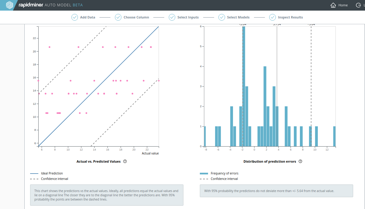
Predicted vs Actual Values Chart: A simple scatter plot of predicted vs actual values shows the performance of the model when applied to the test set. Each point's x-coordinate is its actual value; each point's y-coordinate is its predicted value. The solid blue line y = x represents the placement of points in an ideal (perfect) model where all predictions are equal to their actual values. Dashed blue lines represent the boundaries for x and y of a 95% confidence interval. The closer the points are to the solid blue line, the better the model.
Distribution of Prediction Errors Chart: A frequency histogram of prediction error (difference between predicted and actual values) shows the performance of the model when applied to the test set. A prediction error of 0 represents an ideal (perfect) model where all predictions are equal to the actual values. The more prediction errors near 0 (i.e. the higher the frequency bars near 0), the better the model. Dashed blue lines represent the boundaries of a 95% confidence interval.
Example: Predict sales from advertising data
As an example of regression analysis, we examine the data set Advertising.csv supplied by Gareth James, Daniela Witten, Trevor Hastie, and Robert Tibshirani in connection with their book An Introduction to Statistical Learning. The purpose of this data set is to show that you can predict the volume of sales as a function of advertising budget in three different channels: TV, radio, and newspapers (yes, it's an old data set!).
After downloading the CSV file from the above link, follow the steps outlined in Build models:
Upload Advertising.csv into RapidMiner Go.
Choose "Sales" as the column to predict.
Make sure to select "TV" as one of the inputs. TV advertising has a high correlation with sales, and that will help us to make better predictions.
Select and run all the models.

Model comparison
In the Model Comparison, the Decision Tree is the clear winner when compared to the Generalized Linear Model (GLM):
- It has smaller errors according to each of the metrics Root mean squared error, Average absolute error, and Average relative error.
- It has a larger value for Squared correlation (R2).
The strong agreement between the metrics suggests that there are no significant outliers in this data set.

Decision Tree
By clicking on Decision Tree, you can see the Actual vs. Predicted Values chart. It resembles a straight line, because the predictions are good.

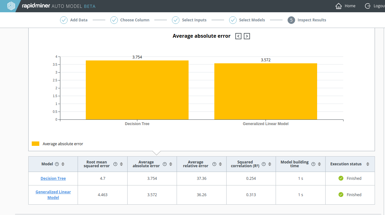
A recalculation: without the TV data
As before, with the Churn Predictive Data, let's do a recalculation where the highly-correlated data is excluded. As the screenshot below clearly demonstrates, the results for the Decision Tree are much worse without the TV advertising data.
- The Average Absolute Error quadruples, from 0.905 to 3.754
- The Squared Correlation (R2) plunges from 0.954 to 0.254
Although it's not good either, the performance of the Generalized Linear Model (GLM) is actually better than the Decision Tree.
Notice that the Actual vs. Predicted Values chart for the Decision Tree no longer looks like a straight line.
Conclusion? To get good results, make sure to include all the relevant data.