You are viewing the RapidMiner Studio documentation for version 2024.1 - Check here for latest version
Interactive Analysis
You need an Altair Units License to use this feature.
You can also see the video guide for an introduction to Interactive Analysis
When you are faced with a binary classification problem using Altair AI Studio, Decision Trees can provide a useful solution. The Interactive Analysis view is an extension to Altair AI Studio that enables you to build a customised node-by-node segmentation model that fit the exact needs of your data. Decision Trees split a dataset based on the relationship between a dependent and an independent variable. Decision Trees are a versatile data mining technique for supervised learning. It also contains a process that you yourself can modify and put into production.
Decision Trees address three large classes of problems:
- Binary Classification
- Classification
- Regression
The Interactive Analysis view helps you evaluate your data with its intuitive and easy-to-use interface, by exploring unfamiliar variables and identifying highly-predictive independent variables that can then be used in other modelling techniques, for example, a logistic regression model.
When using Altair AI Studio, the Decision Trees view appears next to the Design view, the Results view, Turbo Prep view and Auto Model view.
If your data is in a scattered or inconsistent state, not yet ready for model-building, see Turbo Prep.
Example: Predict Survival on the Titanic
To show how Decision Trees work, we'll use the Titanic dataset, included with
Altair AI Studio, to predict survival. This is represented as a binary
variable on this dataset. To get started, choose the Decision Tree view by
pressing the button at the top of Altair AI Studio.
Select Data
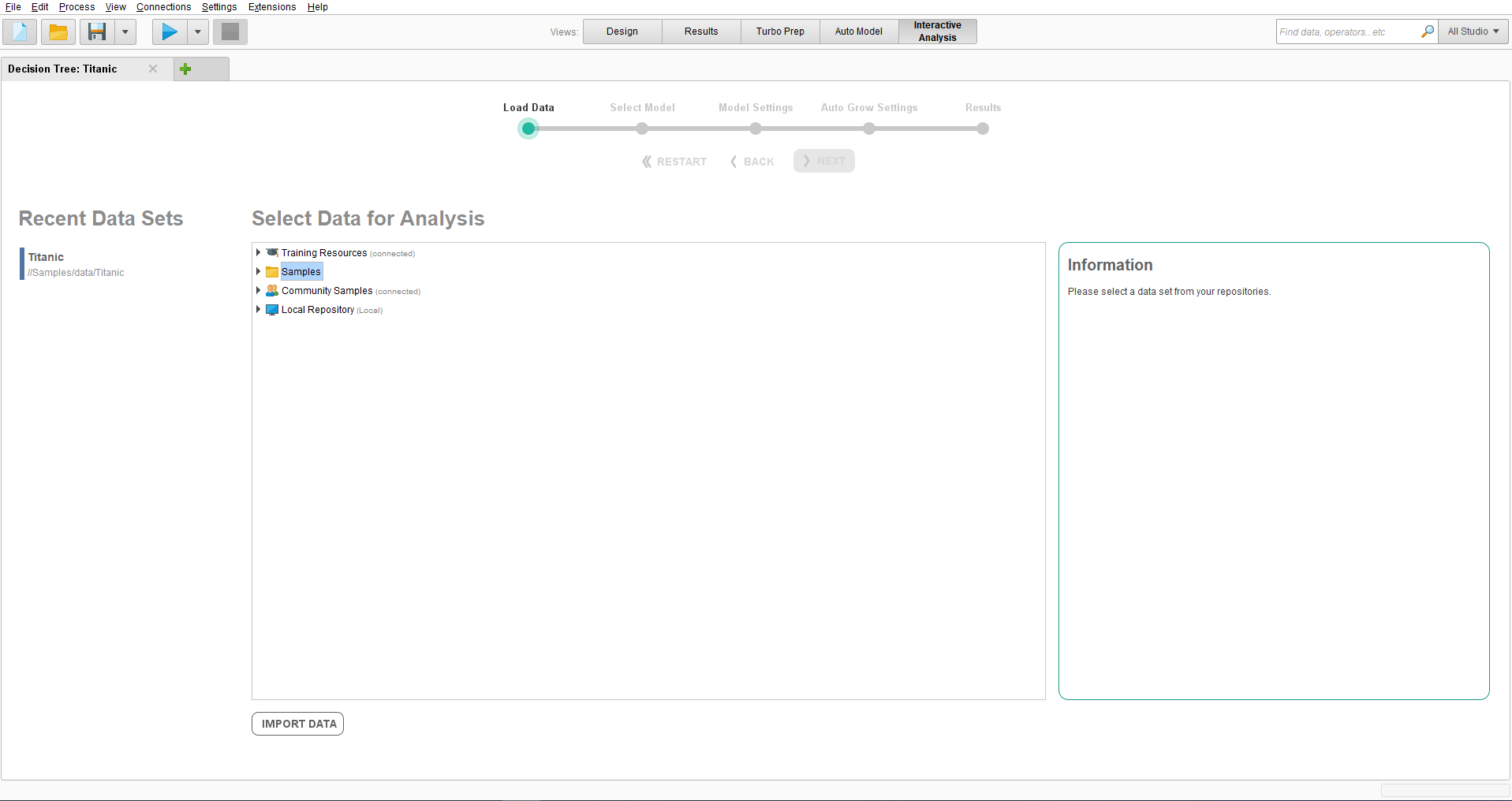
After opening the Interactive Analysis view, the first step is to select the Titanic
dataset from the Samples repository. This can be found under Samples >
data. Select this dataset, then click Next at the bottom of the screen.
Select Model
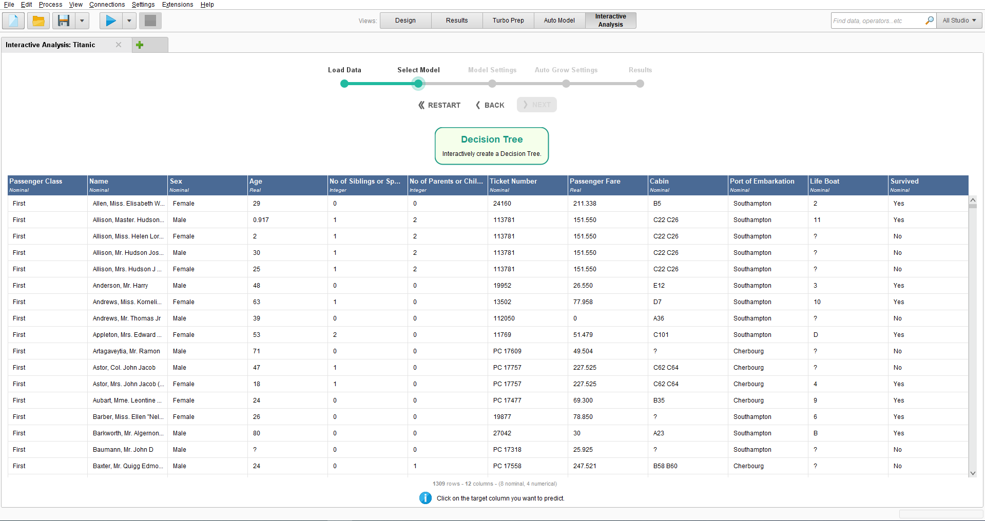
Having selected the Titanic dataset, we want to predict survival on the
Titanic, so you should select the "Survived" column, before clicking Next.
Model Settings
Since "Survived" has only two values, "Yes" or "No", the problem is a
classification problem. In general, for classification problems, Interactive
Decision Tree displays a split report with the number of data points in each
class. If you want to use a specific split search method or criteria you can
select this from the Training Parameters panel using the Split Search Method
list and the Measure drop-down box. You then click Generate Split Report to
refresh the split report.
Split Report
The report in this view generates a report for each variable in the dataset
(excluding the target "Survived" variable) containing univariate information
and information with respect to the target. A data quality report is generated
for each variable that summarises all the information in the Quality column
and based on this, a recommendation is made in the Status column whether the
variable should be included in the model using a traffic light system (red /
yellow / green). The variables with a green status are automatically selected
as dependent variables. There can be a number of reasons why a variable is or
is not selected for modelling. For example, the status on the Ticket Number
column is red as it shows an "ID-ness" of above 70%, that is, the number of
unique values is more than 70% of the total number of rows in the dataset which
would not make the variable a very effective predictor.
Not all of your data columns will help you to make a prediction. By discarding some of the data columns you can speed up your model and / or improve its performance. But how do you make that decision? A key point is that you're looking for patterns. Without some variation in the data and some discernible patterns, the data is not likely to be useful.
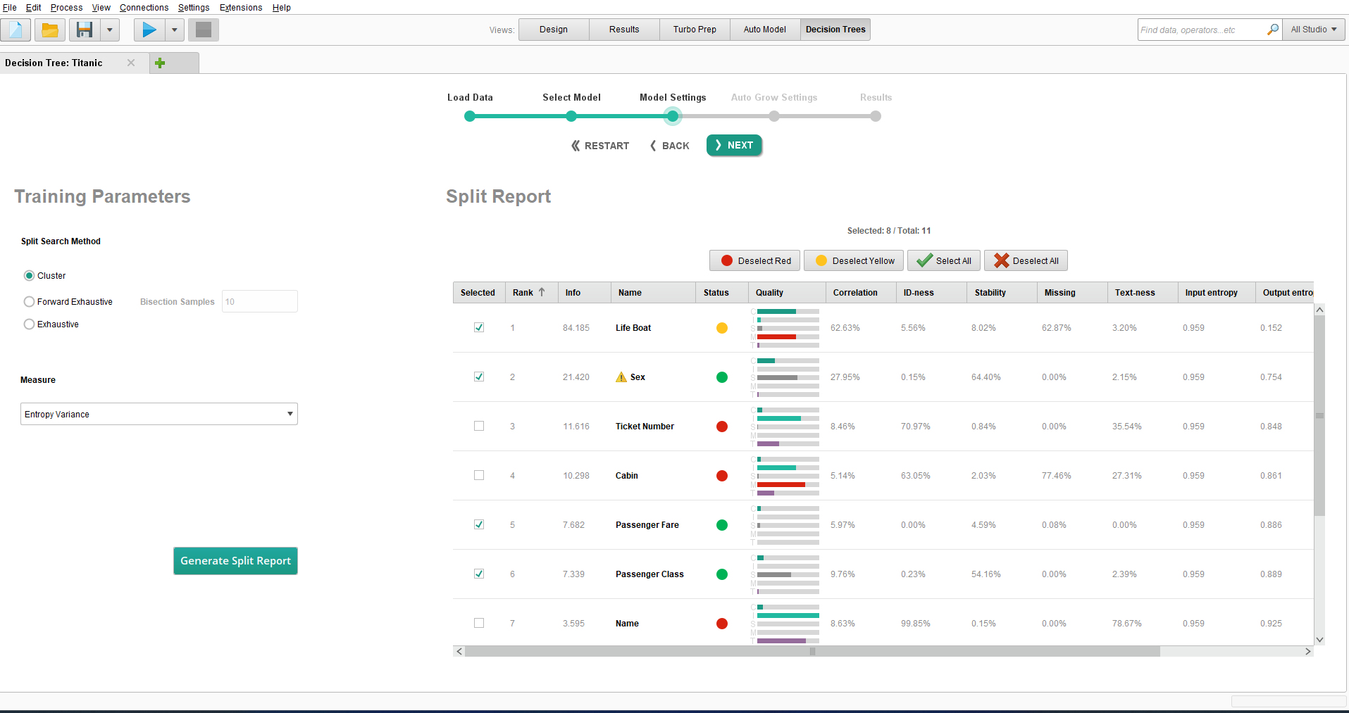
A quick summary of what to look out for includes the following, whose values are displayed alongside the quality bars for each data column.
- Columns that too closely mirror the target column, or not at all (Correlation)
- Columns where nearly all values are different (ID-ness)
- Columns where nearly all values are identical (Stability)
- Columns with missing values (Missing)
The split report summarizes the situation with a color-coded status bubble (red / yellow / green). As a general rule, it is a good idea to deselect at least those columns that have a red status bubble, but of course you can deselect any columns you like, independent of their status. The input for the machine learning model only includes the selected columns.
In the case of the Titanic dataset, the "Name" and "Ticket Number" are equivalent to IDs. The "Cabin" values are missing for most passengers. Hence, these three columns, with a red status bubble, should be discarded when building a model. None of them is helpful in discovering a pattern.
"Life Boat" has a yellow status bubble, because the data in this column is highly correlated with "Survived". "Lifeboat" and "Survived" are effectively synonyms, so it is better to remove the data from the "Life boat" column and let the model discover the underlying reasons for survival.
You want the model to create a plan; A passenger can't know in advance whether they will be on a lifeboat, so that can't be part of the plan, but they can decide how much to pay for their ticket, and whether or not to bring their family along.
In this example, you should also deselect the data with the yellow status bubble,
"Life Boat", and press Next.
Auto Grow Settings
Having selected the variables for the model, we now configure the growth settings of the Decision Tree. A Decision Tree begins at a base node that represents the entire dataset, usually a training dataset.
It is good practice to partition your dataset beforehand into a training dataset, which you can use to train the model, and a testing dataset, which you can use to check the accuracy of the model on unseen data. You would ideally like the model to have the same level of predictability for both the training dataset and testing dataset. If the predictions on your training dataset are more accurate than your testing dataset, you are overfitting the model and you might want to either decrease the proportion for the training dataset or resample.
The base node of the training dataset is then split by a variable into further nodes, the split is based on the variable. For example, a binary variable will split the base node into two nodes, these nodes can then be further split by another variable. Nodes are split by variable values if they are binary or discrete, continuous variables are split by one or more inequalities.
With these interactive Decision Trees, you can choose to either grow a tree yourself from the base node or have a tree grown for you. In the latter case, you would still be able to grow individual trees.
There are parameters you can set for the tree under Tree Settings. For all columns you can set the P-value that specifies a p-value for grouping values,
the Max Branches to set the maximum number of nodes to split a base node into, or the minimum number of values for treating a variable as continuous using Min Cardinality for Continuous, you can also
clear Break Apart to create a fast but less accurate decision tree that uses variables with many discrete values.
For norminal (discrete) variables you can set the maximum number of bins (how many nodes you can split from the base node) by entering a value in Max Bins and specify the treatment of missing values using Missing Values. For continuous variables you can set the maximum number of intervals (how many nodes you can split from the base node) and specify whether those intervals are static or dynamic in Interval Type, you can also specify the treatment of missing values using Missing Values. For ordinal variables (discrete and ordered) you can specify the the values displayed in the node in Ordered Display by selecting Rangeto show a range, Present to show the current values in the node or All to show the range and whether those values are present, and the treatment of missing values using Missing Values. For missing value treatment
you can specify Use to include missing values in the split, Ignore to ignore missing values, or Float to ignore missing values when calculating the variable split, then place in a bin after calculation if the p-value set in P-value for merging values is satisfied.
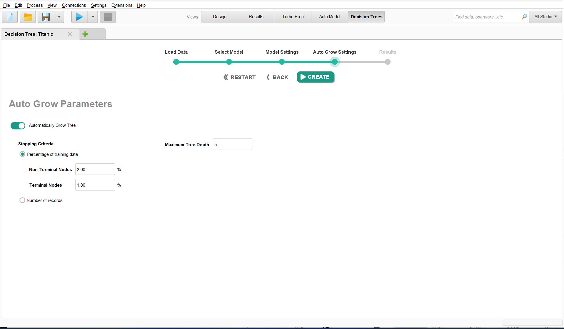
In our example we will start with an automatically grown tree, so ensure Auto
Grow Tree is selected. The settings enable you to specify the restrictions
when automatically growing the tree. You can specify the minimum amount of
data in each node in Percentage of training data and the amount of levels the tree can
deviate from the base node in Maximum Tree Depth In this example we will keep
all the default values and click Create.
Results
Depending on your dataset and the models you selected, you might have to wait for the results. The progress bar at the top tracks the status of an ongoing calculation.
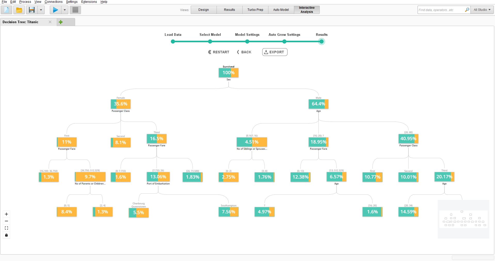
Once the results are ready, the decision tree is displayed in a canvas
containing a view of multiple nodes, all representing a portion of the dataset
shown in the percentage of the node. The base node is representative of the
whole dataset so the proportion is always 100%. Each node also has a colour
coded blue/orange split representing the proportion of the target variable;
you can hover over a node to see the exact number. You can make the canvas and nodes
larger by using the scroll wheel or the + and - buttons on the bottom right of the canvas view.
Increasing the size can change the colour coding of each node to instead show information of the exact number
and proportion of the target variable split and a bar chart, if you want to preserve the colour coding of each node when
increasing their size, click the Settings button on the bottom right and select Full Node Coloring.
If you didn't choose to automatically grow the tree, you can do this manually by clicking on a root
node (a node that isn't already split up) and selecting the Find split button on the
left to split the node by one level or the Auto grow button in the middle to
fully split the node. If the node is already split up, you can make this a root node
again by clicking on it and selecting the Remove child nodes button. A node is split by
the values of single independent variable, this can be by select values if the variable is discrete
or by inequalities if the variable is continuous. You can change the independent variable that splits
the node by selecting a split node and clicking the arrow keys on either side of the variable name. You
can change the split values of the independent variable, to do this, click the Edit button to open a Range Editor window,
select Break for any required values and click Save Range to close the Range Editor window. You
can also view a split report for the variable by selecting the View split report button.
In our example the Decision Tree is already fully grown out, from here we can gain insights about the data: The first level splits the data up by gender and we already find the target variable proportion is quite split between females and males with 19% of males surviving compared with 73% females. The female node is then further split by passenger class to show that 96% in first class survived, then 89% in second class and finally 49% in third class. The male node is further split by age with 51% surviving ages 0-18, 12.5% ages 18-20 and 19% ages 20-80. We can understand from this that first class females on board were very likely to survive, while adult males were much less likely. If we were to apply the model to some data, each data point would run through the tree and run through the value of each variable specified in the tree until it reaches one of the end nodes. From the end nodes a probability is then returned that is the target variable proportion in that node. The returned probabilities can make predictions by splitting the <0.5 and ≥0.5 probabilities into its own binary variable. This binary variable will then serve as the model prediction, for example a Decision Tree model of the Titanic dataset can make a variable that predicts a ≥0.5 chance of survival to survive and a <0.5 chance to not survive.
You can export the Decision Tree canvas as an image, to do this, click the hamburger icon
on the right of the canvas and either select Export as PNG or Export as JPG, then save the image in
the required location.
The Decision Tree model can be exported from this view and applied into an
Altair AI Studio workflow; to do this, click the Export button to open the
Export Model dialog box then select a repository folder and name the model in
the Name text box then click Next. Once the model has finished exporting
click Close to close the Export Model dialog box. Your Decision Tree model
is then ready to use in the Altair AI Studio Workflow.