You are viewing the RapidMiner Studio documentation for version 9.5 - Check here for latest version
Deployments
Introduction
See also the video introductions to Model Operations: Introduction / Deployment / Management
To realize the full value of your models, you have to put them into production. In the guided approach provided by RapidMiner Studio, that means:
Preparing your data with Turbo Prep
Building your models with Auto Model
Deploying your models in the Deployments View ("Model Ops")
From within Auto Model, you can deploy a model with a single click!
A deployment is a collection of models describing the same input data. In its simplest form, it lives in a repository and scores data (e.g., makes predictions), but it can do much more!
- A deployment organizes your models and keeps essential data together in one place (e.g., for compliance with regulations such as GDPR).
- A deployment tracks the performance of your models over time, alerting you to drift and bias.
- A deployment can be shared by a group collaborating on a common project.
- A deployment provides web services, so that you can integrate it with your other software.
A deployment location is a container for one or more deployments.
- Multiple deployments can be stored in a common deployment location.
- Teams working separately can have different deployment locations.
The basic philosophy is: the more models you can get into production, the better. Therefore, deployment should be as easy as possible. Why let your models go to waste?
Jump to the Table of contents
Plan your deployment
A deployment location is to start with an empty folder, either local or remote. The best policy, once you have created this folder, is not to touch it, to avoid breaking your deployments.
| Deployment location | Folder location |
|---|---|
| Local | RapidMiner Studio repository |
| Remote | RapidMiner Server repository |
A deployment location on RapidMiner Server can be shared, and you can control access by appropriately configuring users and groups.
If you are not careful when planning your deployment, you may discover afterwards that it is lacking crucial components. Notice that:
- monitoring helps you to collect long-term scoring statistics. To activate monitoring, you have to create a database connection.
- remote deployment allows you to share the deployment and to integrate the deployment with other software.
Make sure to create an appropriate deployment location.
Components of a deployment
Within a deployment location, you create a deployment. That deployment will provide a subset of the following components, depending on the context of the deployment location.
If you create a remote deployment with monitoring, the full set of components will be available.
| Component | Description |
|---|---|
| Dashboard | Displays scoring statistics, measured over time |
| Models | A list of competing models, built on the same or at least similar data sets (same columns and same data types), where one model is active and the remainder are challengers. For compliance with regulations such as GDPR, full details of each model are included, including the original input data set and the process that was used to build the model. |
| Performance | Displays detailed scoring statistics, per model, measured over time |
| Drifts | The difference between the input data distribution and the distribution of the scoring data. The difference may occur either because of bias -- because the input data was not representative -- or because the scoring data has drifted. If the measured drift is significant, you may want to rebuild your models. |
| Simulator | The model simulator, as known from Auto Model |
| Scoring | An interface to upload the data you want to score and to review the results |
| Alerts | An alert warns you when there is unusual or undesired behavior in your deployment |
| Integrations | Web services make it possible to share the deployment and integrate it with your other software |
By default, every deployment location includes Models, Simulator, and Scoring. The table below describes the additional components that become available when:
- you activate monitoring,
- you create a remote deployment location
| RapidMiner Studio | + Database Connection | |
|---|---|---|
| RapidMiner Studio |
|
|
| + RapidMiner Server |
|
|
Create a deployment location
To create a remote deployment location, you need access to a RapidMiner Server repository.
The following screenshots illustrate the creation of a remote deployment location, with monitoring. The steps for creating a local deployment location are mostly the same. Where the situation is different, we make a comment.

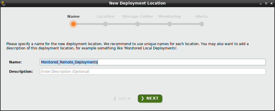
From within the Deployments Overview, click New to add a deployment location, and enter a name in the resulting dialog. In our example, we write "Monitored_Remote_Deployments", and click Next.
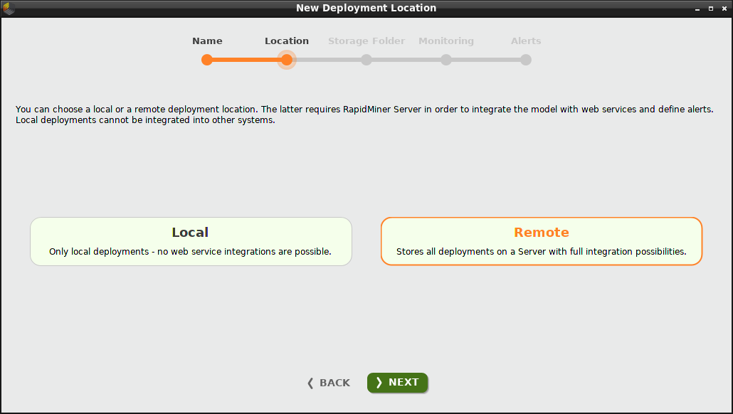
We choose to create a Remote deployment location. The deployments in this location will include alerts and integrations. In contrast, a Local deployment location does not include these components.
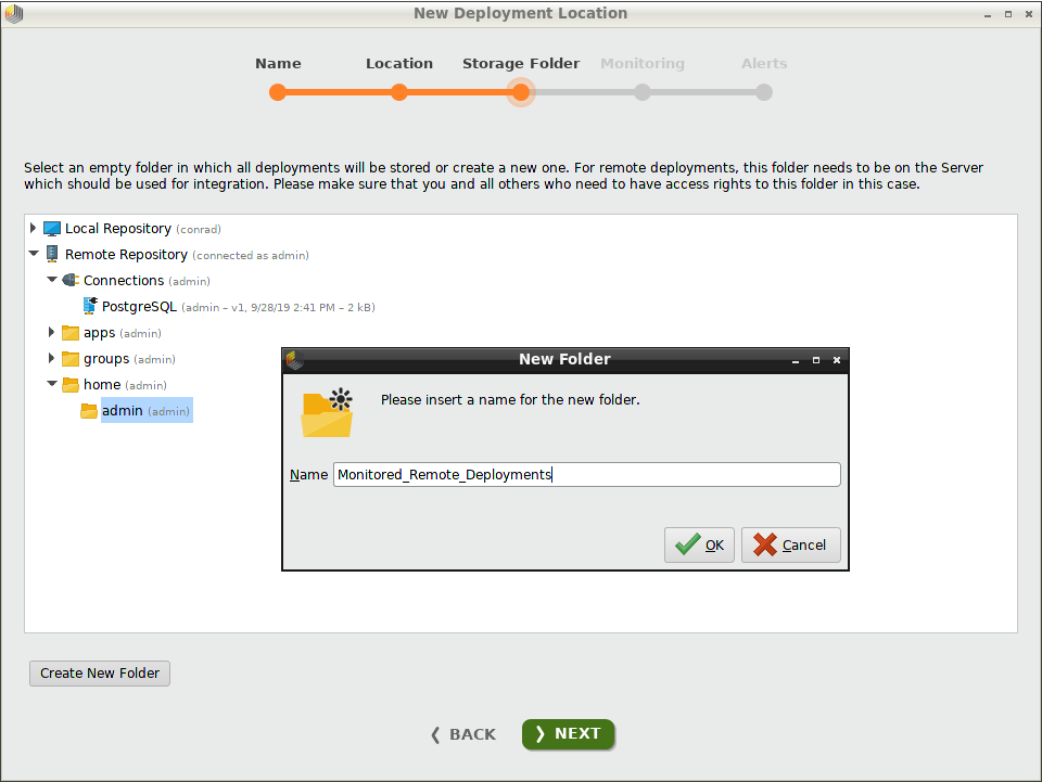
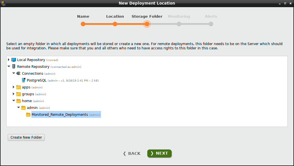
If you have not yet created an empty folder inside the repository, you can
click Create New Folder. In this case, we create and select a folder
called "Monitored_Remote_Deployments" inside the "Remote Repository", under /home/admin.
You can create the folder anywhere you like, so long as it is empty.
Notice that this repository includes a "PostgreSQL" connection, which we will need when we activate monitoring.
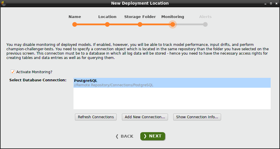
To activate monitoring, you need a database connection.
To activate monitoring, click the checkbox and select a database connection. Click Add New Connection if you need to create a connection. In our example, we select a pre-existing "PostgreSQL" connection.
Thanks to monitoring, all the deployments in this location will include a dashboard and summaries of performance and drifts. Without monitoring, these components are not included.
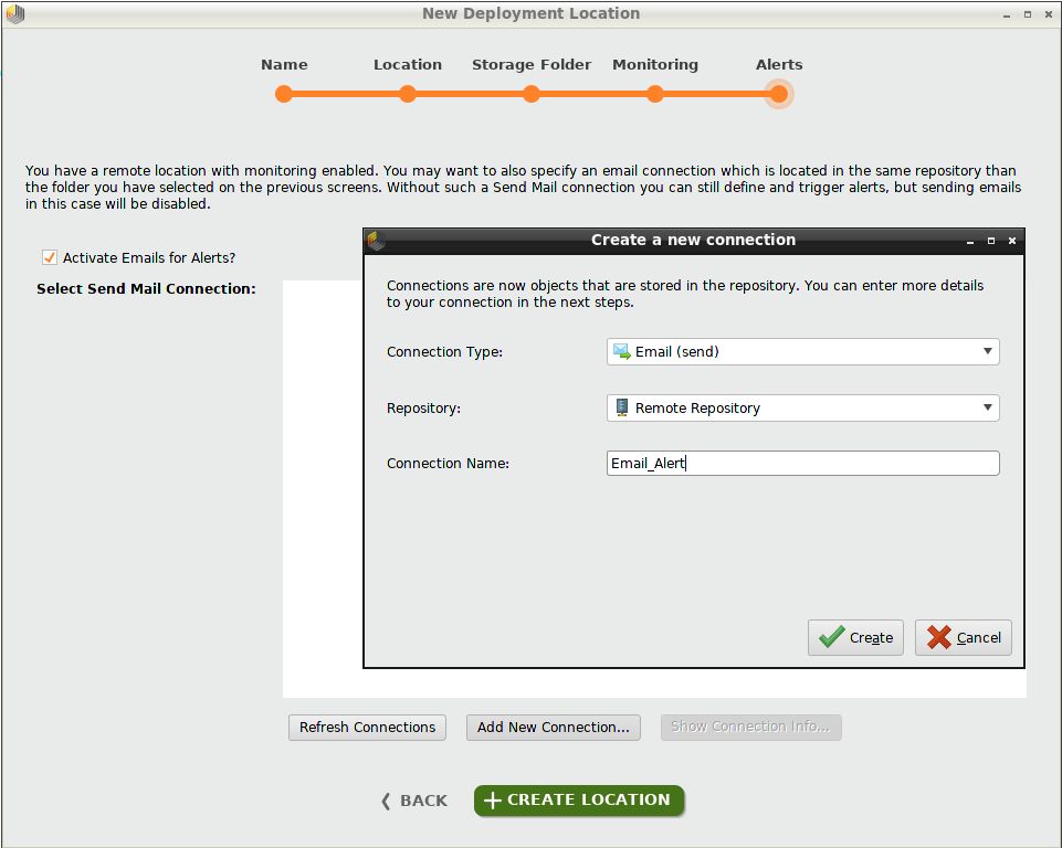
To create alerts, you need a remote deployment location and you need to activate monitoring.
To activate email alerts, click the checkbox and select a Send Mail connection. Click Add New Connection if you need to create a connection. In our example, we create and select an Email connection called "Email_Alert".
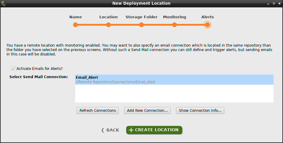
Click Create Location, and you're ready to add deployments! The deployment location we just created appears in the upper right corner of the overview, in a drop-down list together with any other deployment locations.
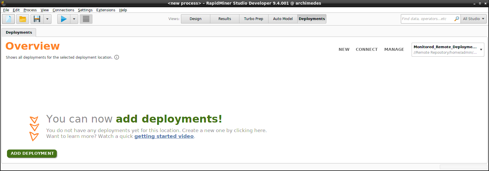
From within this Deployments Overview, you can Add new deployment locations, and Manage your existing deployment locations.
Create a deployment
At this stage you can click Add Deployment and create a deployment, but that deployment will have no content until you add some models. We create a deployment called "Churn", and identify our problem as a classification problem, before proceeding to build the models using Auto Model.
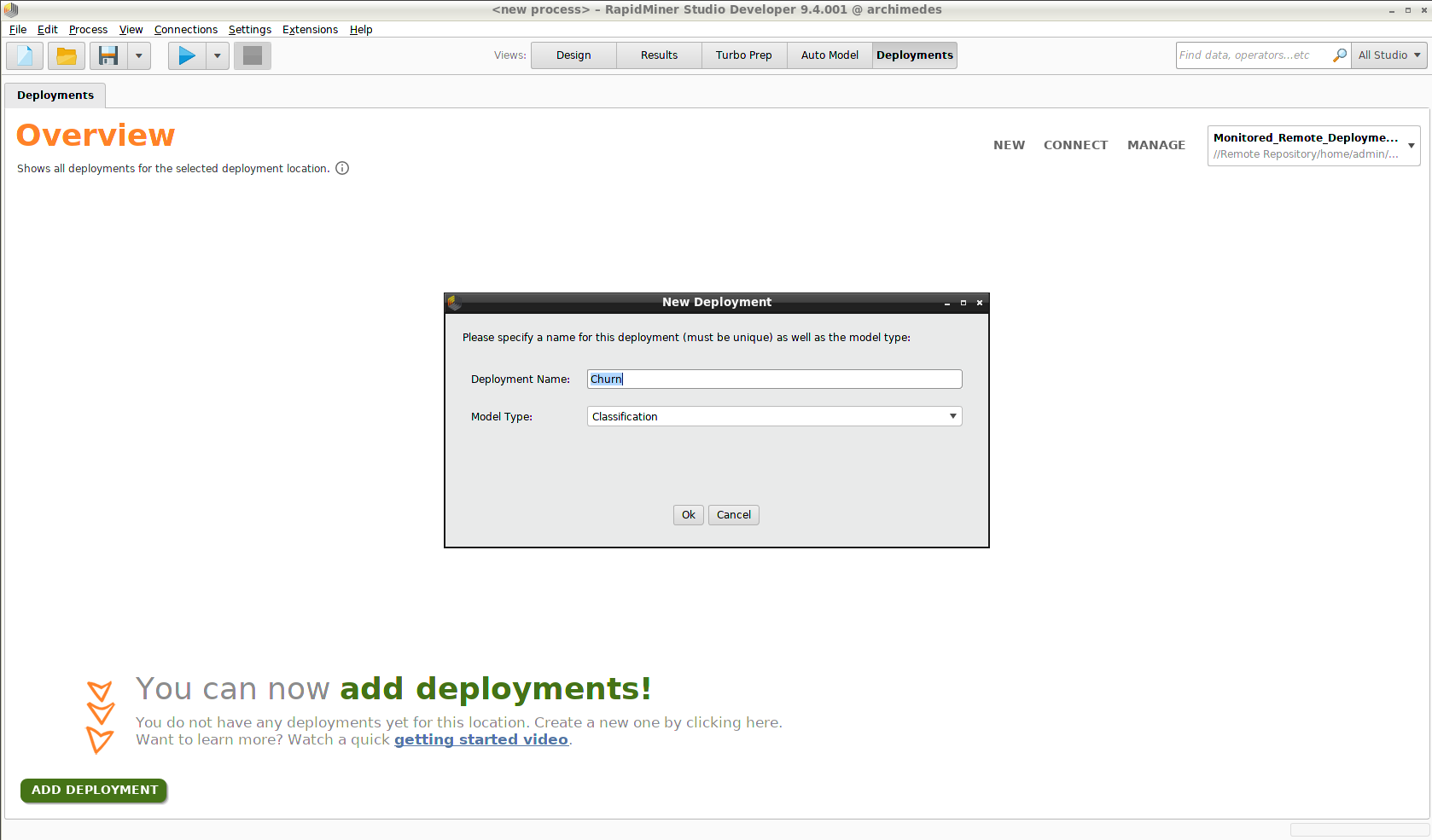
Example: Churn
To provide the content for our deployment, we use a data set provided in the Community Samples repository, under Community Samples > Community Real World Use Cases > TelCo Customer Churn, using part of the data set for modeling, and the rest to simulate scoring.
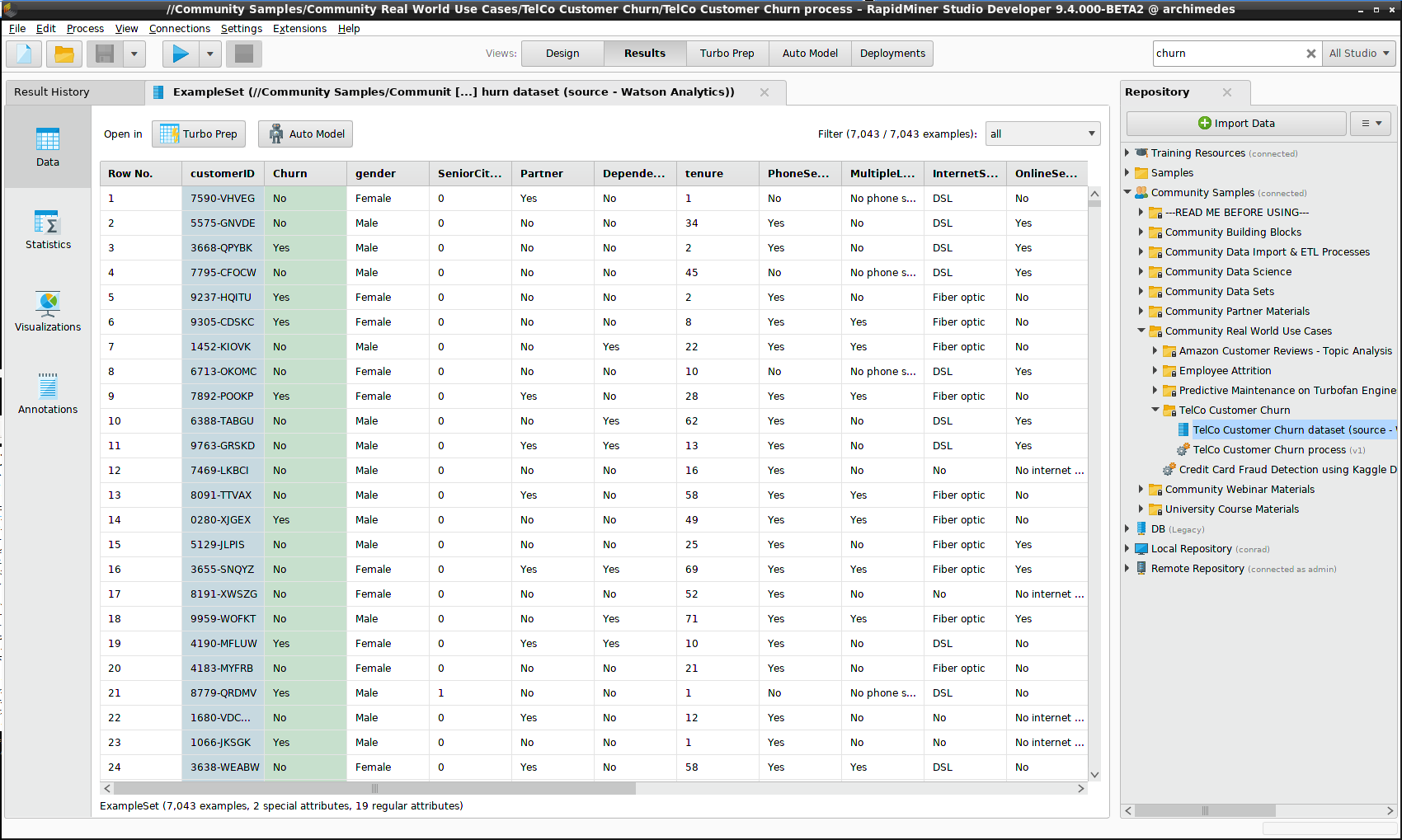
The issue here is not merely to predict which customers of the phone company will drop their subscriptions, but to calculate the gains achievable by the model if it can correctly identify the churners, assuming that the phone company can retain them via a rebate.
Gains
As an option, Auto Model includes a performance metric that allows you to assign a cost to every element of the confusion matrix, so that the results are no longer identified as merely true or false, but in terms of profit and loss.
During the creation of the models with Auto Model (Prepare Target), we press the button Define Costs / Benefits, and a dialog opens. Costs are identified as negative numbers, and benefits as positive.
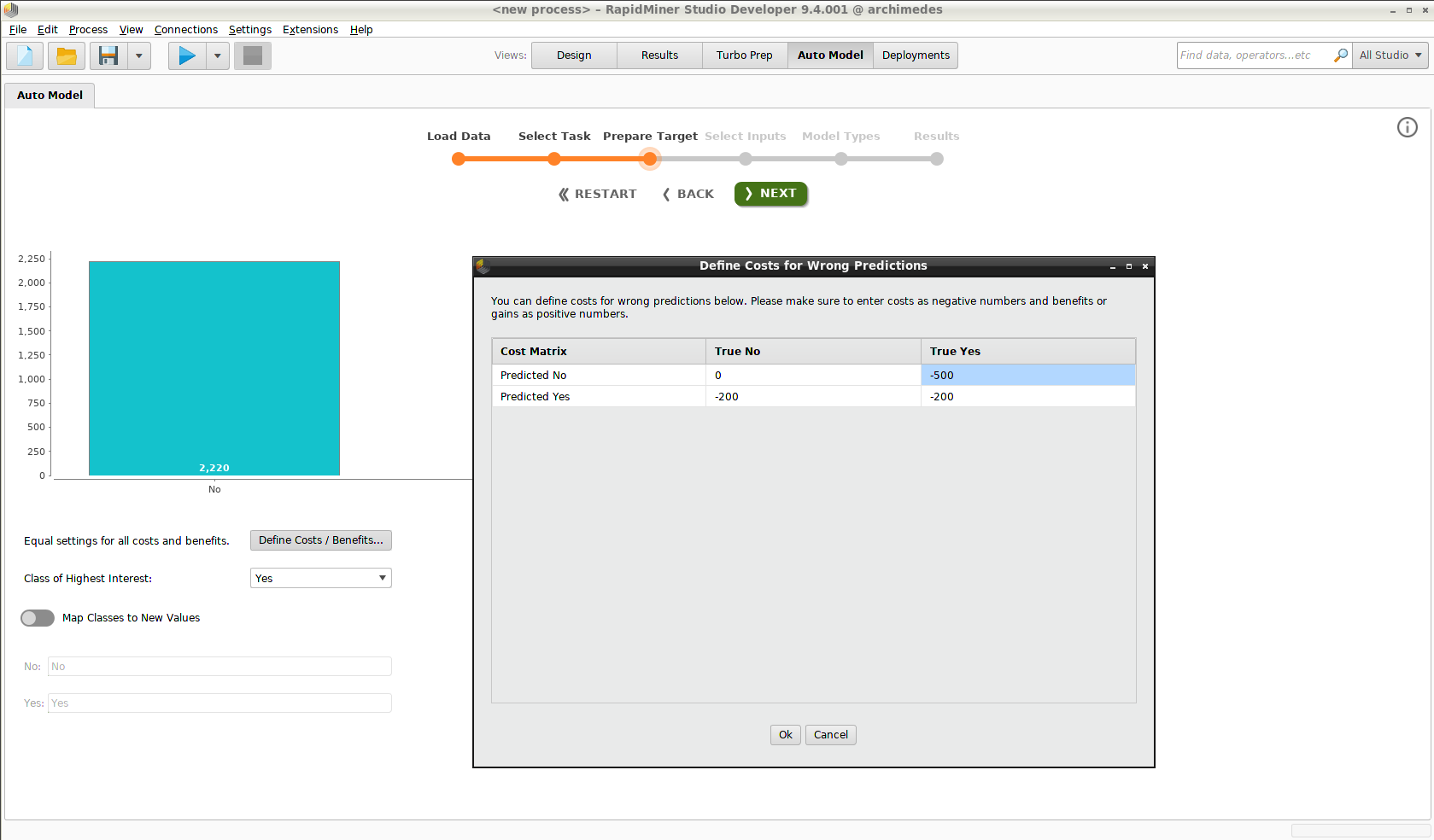
- The default situation, with zero cost or benefit, is that the customer keeps his subscription.
- A customer who is identified by the model as a churner will be offered a rebate worth $200 to convince him to stay.
- A false negative (the model predicts the customer will stay, but he churns) is a worst case scenario. We assume that with the rebate, he would have stayed. Therefore a cost of $500 dollar is assigned to that element of the matrix, the revenue associated with a lost customer.
Using these values, we can calculate the cost of applying the model, and compare it to the baseline cost, according to which every customer who churns (with no rebates offered) represents a loss of $500. The gain provided by the model is the difference between these two calculations.
In the sections that follow, including Scoring, Dashboard, and the Performance summary, the costs / gains associated with the model will be included when presenting the results.
Auto Model
The procedure for building a set of models was discussed previously in Auto Model. Our current example is no different, except that we have defined a cost matrix as discussed above. After accepting all the defaults and creating the models, we arrive at the Auto Model overview.
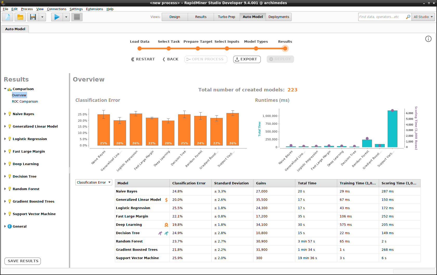
Any or even all of these models can be included in our "Churn" deployment by clicking on the model in the side panel, choosing one of the submenu items, and then clicking Deploy.
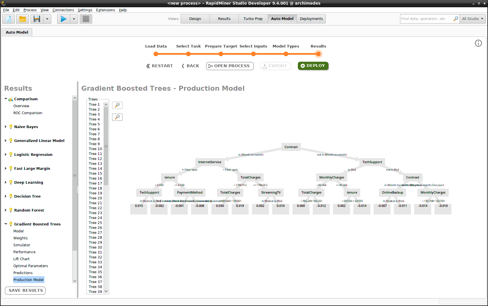
Deploy the model
Deploying the model consists of three steps.
Name the model (e.g., "Gradient Boosted Trees")
Choose the deployment location (e.g., "Monitored_Remote_Deployments")
Choose the deployment folder (e.g., "Churn")
If you have not yet created a deployment location or a deployment, you can do so during this process.
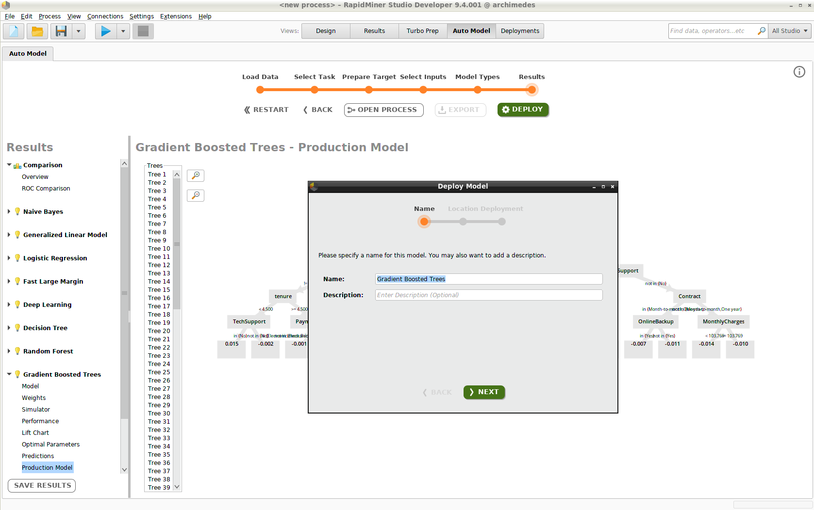
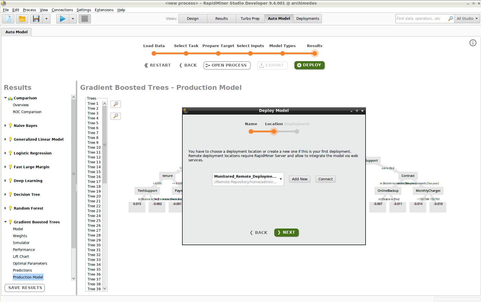
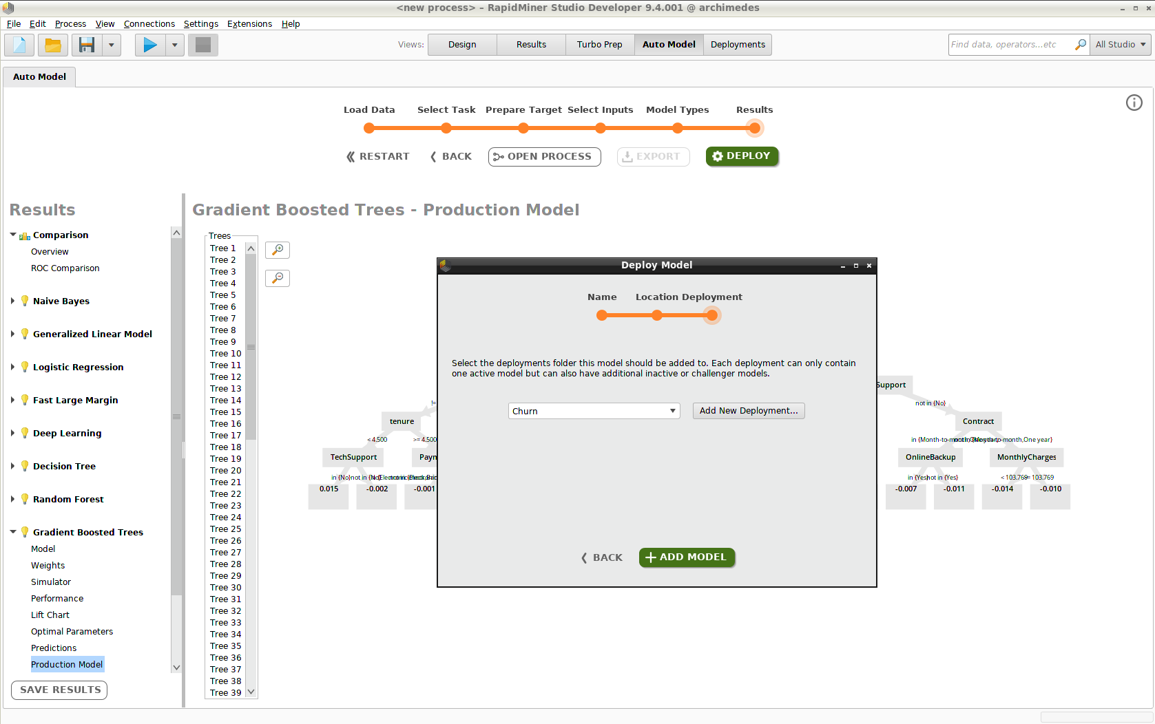
Click Add Model, and the model appears in the Deployments View. To include additional models in the deployment, you have to return to the Auto Model View.
Models and Scoring
This section and the following sections discuss the components of a deployment in greater detail.
The essential components of any deployment are models, the model simulator, and scoring. If you want not just to score data, but to calculate statistics for your scored data over time, you should in addition activate monitoring.
Models
Usually, a deployment will contain multiple models. Ideally, you want to use the model with the best performance, but you can't exclude the possibility that the situation will change over time, as the world changes and your input data drifts.
One model should be marked as Active, while the remaining models are marked as Challengers. The choice of active model is at all times up to you; you might choose the model with the best performance or the the model with the fastest scoring times, for example. Every time you use the deployment to score new data, both the active model and the challengers calculate the results. If, at some later stage, you decide that one of the challenger models better suits your problem, you can replace the active model.
Notice that in the example below, the Generalized Linear Model had the best performance when the models were built, before deployment, but it has since been superseded both by Deep Learning, marked in green because it is doing better than expected, and Gradient Boosted Trees, marked in yellow because it is doing slightly less well than expected. Both Naive Bayes and Decision Tree are doing poorly. If these models continue to perform poorly, you may want to mark them as Inactive, so you don't waste Scoring Time.
Since Gradient Boosted Trees has better performance than Deep Learning, we right-click the model and select Change to Active.
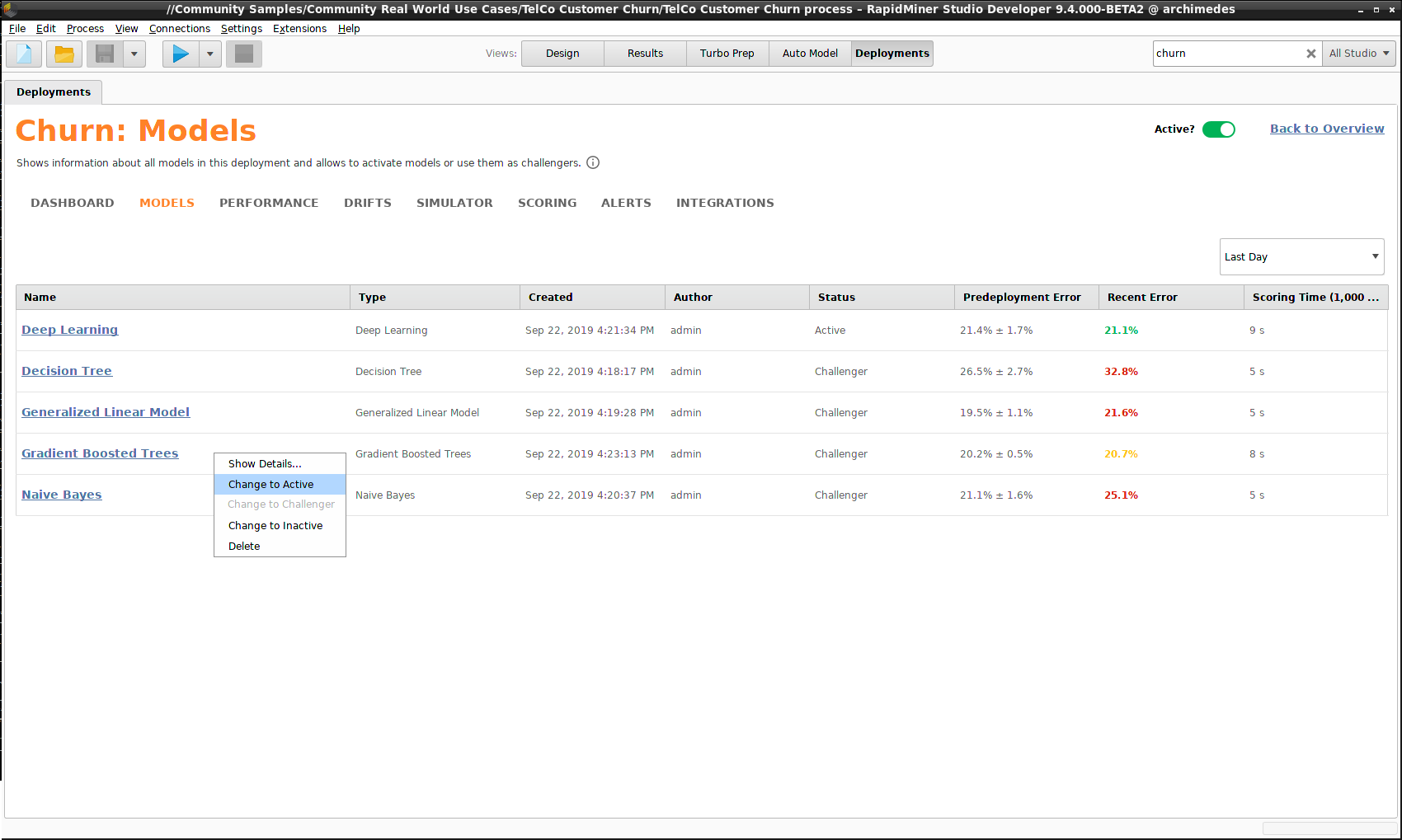
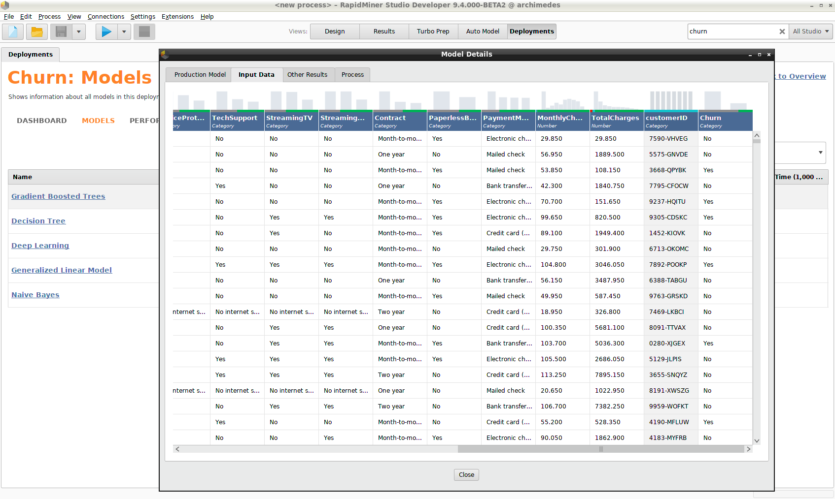
If you right-click any model and select Show Details, you will see that the model contains, among other things:
- The complete Input Data set that was used to create it
- An XML representation of the Process used to build the model
For compliance with regulations such as GDPR, this information is essential.
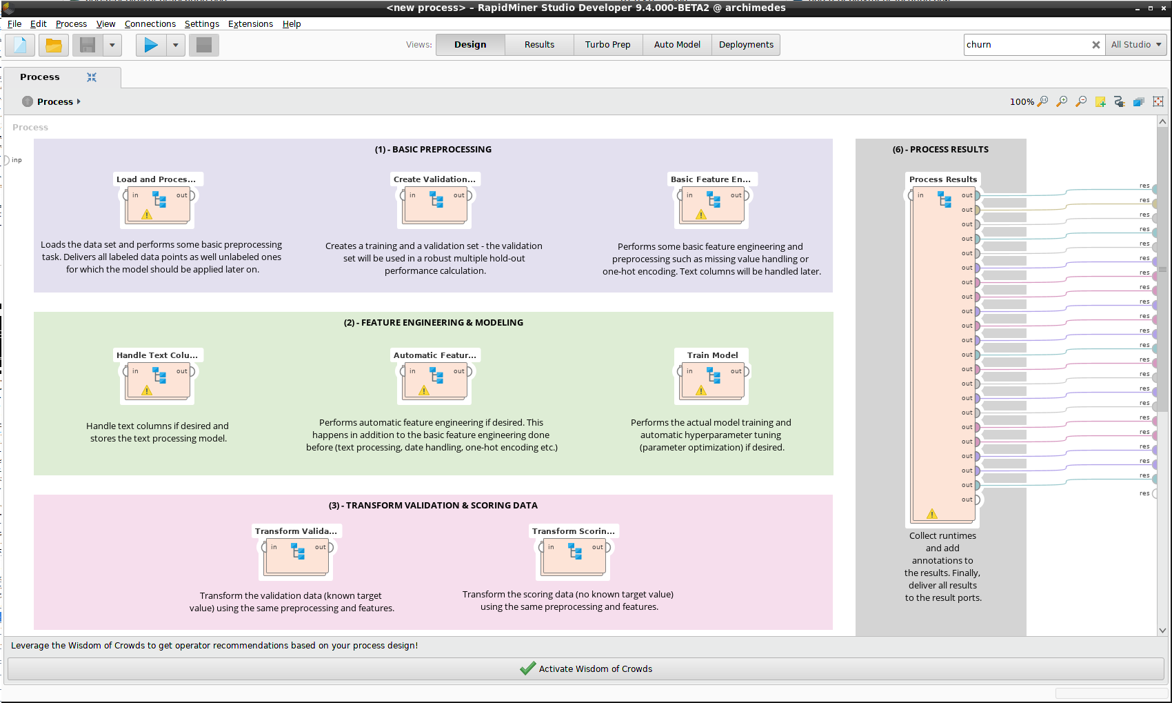
An annotated version of the Process can be displayed in the Design View.
Simulator
The model simulator is described in more detail in Auto Model. The simulator attached to each deployment is the simulator belonging to the active model.
Scoring
For a programmatic approach to scoring data, see integrations.
Arguably, the main purpose of a deployment is to score data. Your models take new data as input, and return a result. If you have activated monitoring (highly recommended!), the results are collected so that you can keep long-term statistics.
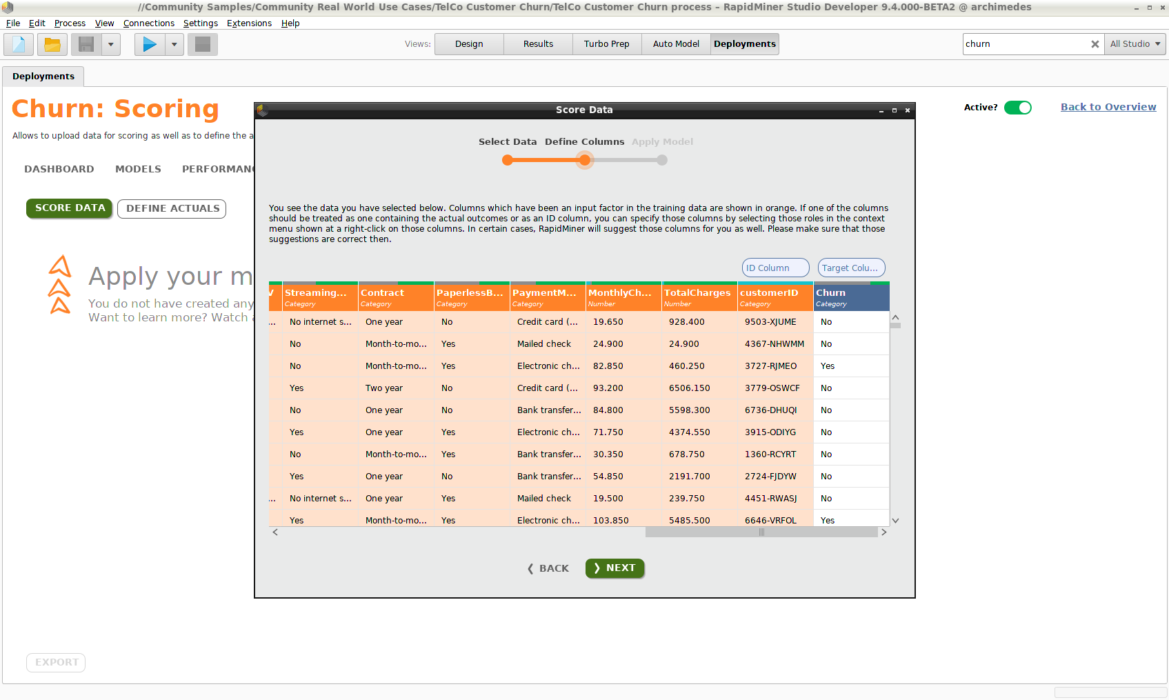
Click Score Data, and choose a data set from the repository. Note the following points.
- The scoring data set should contain columns similar to the data set that was used to build the models. The scoring process is robust enough to accept data types that are slightly different, so long as they both have the same supertype (e.g. real or integer, since both are numeric). The process can also detect changes in the column name, so long as the data type and distribution resemble the input data.
- Data columns that were not included when you built the model will be ignored.
- Data columns that are required by the model, but missing, will be supplied, using mean values or the mode.
Two columns of data have a special status:
- Target column - If the target values of the scoring data are known, they can be compared with the predictions to generate statistics for the models' error rate. Often you won't have this information at the time of scoring (that's why you need a prediction!), but you can add it later if you can identify the data via an ID column.
- ID column - If you lack a Target column in your scoring data, but you have an ID column, you can resubmit the data with the same ID later, when the target values are known, to generate error rates and other statistics. Click Define Actuals to resubmit the data.
When you submit your scoring data, an attempt will be made to identify the ID and target columns. Even if these columns are identified incorrectly, you can assign the correct values by right-clicking the affected columns and choosing Use as ID or Use as target. Only columns that are not used by the model as input can be identified as ID or target columns.
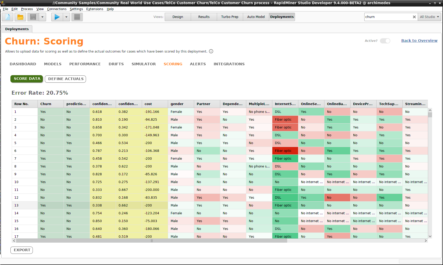
The results are returned as a table with some additional data columns:
- prediction
- confidence values
- costs
Since in our example the scoring data included target values, the error rate is calculated. Note that you can Export the results to a file or a repository.
If when you ran Auto Model, the checkbox Explain Predictions was checked, the scoring data is color-coded to indicate its importance for the prediction: dark green values strongly support the prediction for that row of data, dark red values strongly support a different prediction for that row of data, and lighter colors are less important.
Monitoring
To activate monitoring, you need to create a database connection. Currently, only MySQL and and PostgreSQL are supported.
Note that the Model Operations database is independent of the RapidMiner Server database; if you have installed a RapidMiner Server database with MySQL or PostgreSQL, you can use the same database, but there is no need to.
Every time you score data, you get a result. You could manually collect all the results and analyze them, but there is a better way.
If you activate monitoring, the scoring statistics are collected for you, so that you can check that everything is working as expected. Monitoring helps you to answer the following questions:
- Are you regularly scoring data? How much data?
- What is the error rate of your models?
- How much have you gained by applying the models to your data?
- Is the distribution of your scoring data consistent with your models (Drifts)?
- Have unusual events triggered any alerts?
- What is the average response time when you score data?
The answers to these questions are displayed cumulatively in a Dashboard and in greater detail (per model) in the Performance summary.
Dashboard
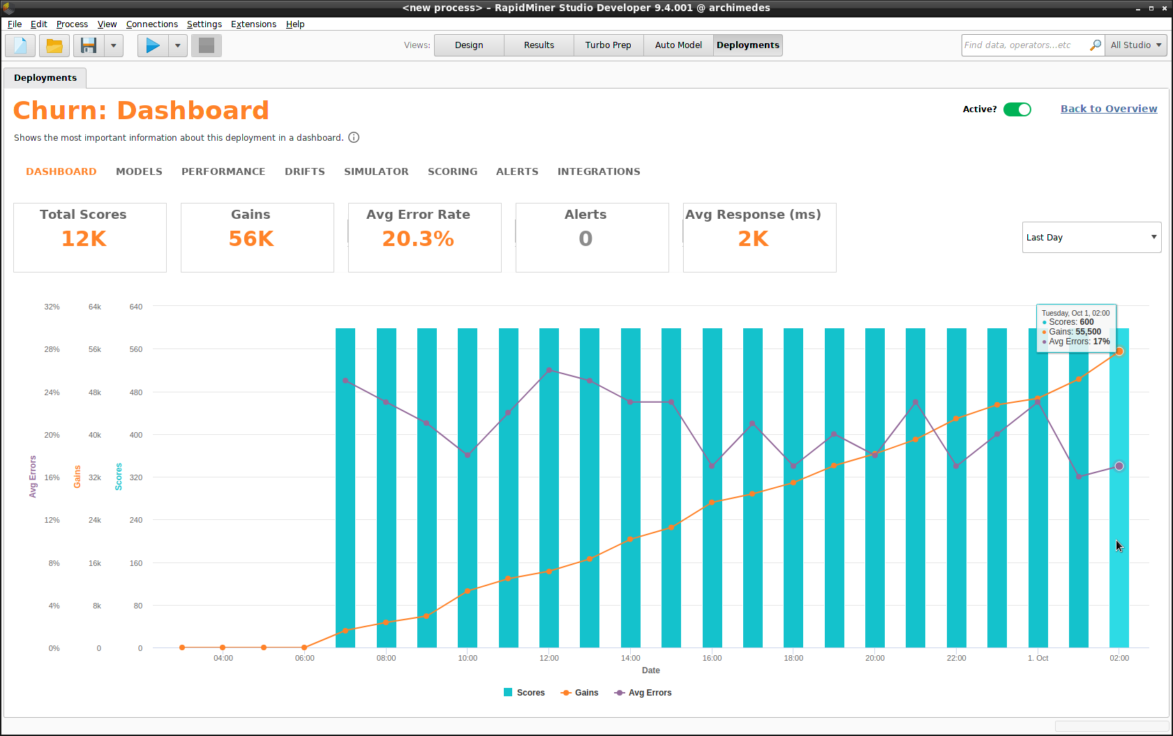
The Dashboard provides the following statistics, displayed over time. You choose the time interval: daily, weekly, monthly, or quarterly. For more detail, see the Performance summary.
Performance
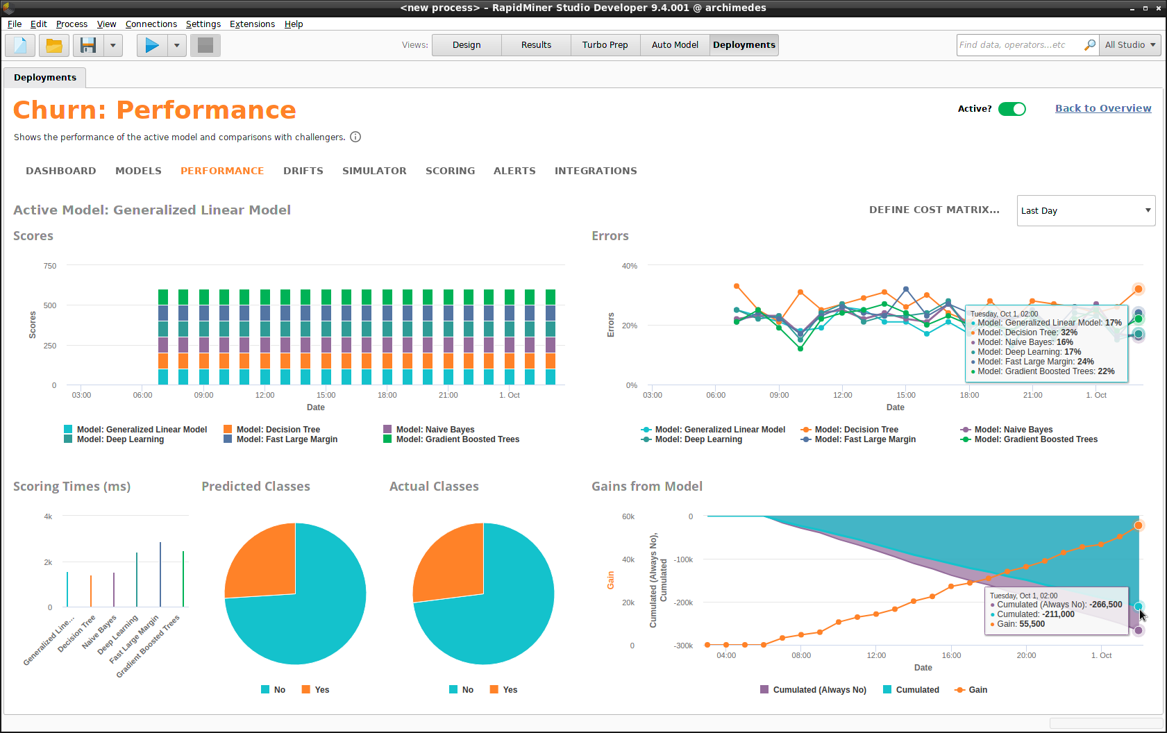
The Performance summary provides even more detailed statistics than the Dashboard, displayed per model, over time. You choose the time interval: daily, weekly, monthly, or quarterly. The Performance summary is the heart of your Model Operations.
- Scores
- Errors
- Scoring Times
- Predicted Classes versus Actual Classes
- Gains from Model
Notice that by clicking on Define Cost Matrix, we can redefine the cost matrix that we created earlier, leading to a revised chart in Gains from Model.
Drifts
For every column of input data that was used to build the deployment models, there is a unique distribution of values. While there is no reason to expect that the scoring data will be identical to the input data, the success of your models to some extent depends on the stability of these data distributions. When the scoring data has a different distribution than the input data, it is called drift.
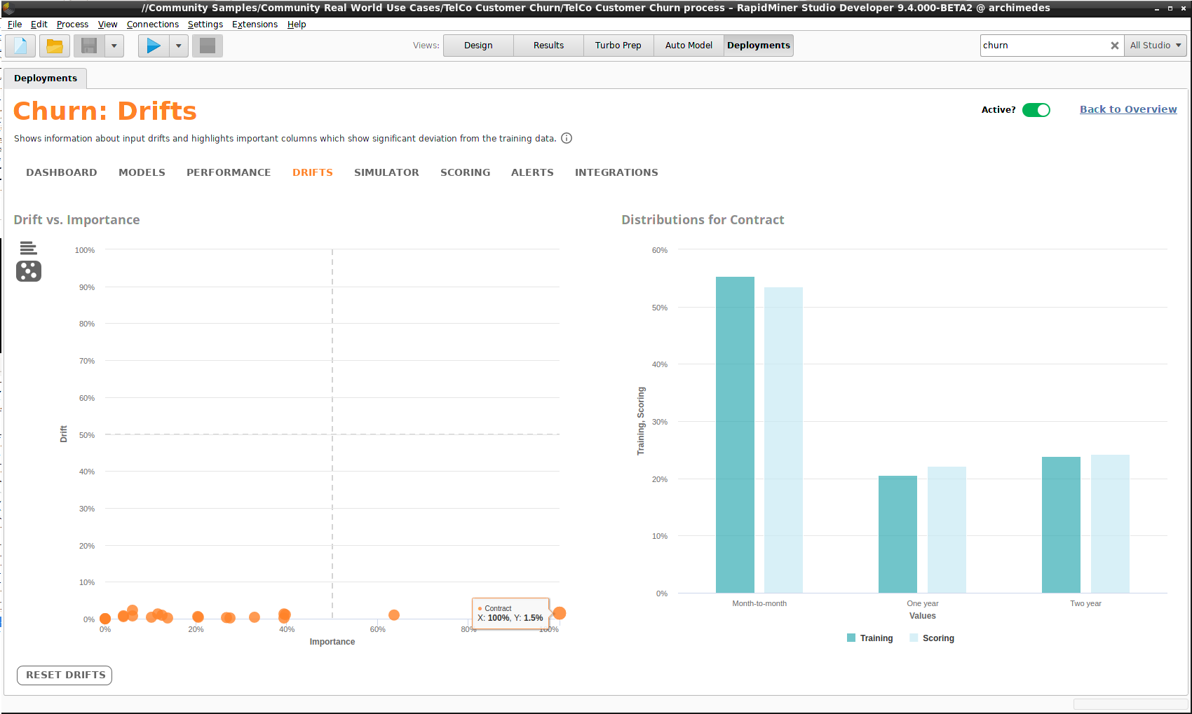
Drift is not unusual; the world changes, and so do your data distributions. But if the changes are significant, you should rebuild your models. How do you know if the changes are significant? The Drifts component helps to provide an answer. For every column of input data, Drifts compares its distribution with the distribution of the scoring data. There are two charts available:
- Drift for Factors - a bar chart, with column names ordered by the amount of drift. Click on a bar to see the distributions.
- Drift vs. Importance - a scatter plot, measuring drift versus importance for each column. Click on a point to see the distributions.
The problems occur when a column that plays a significant role in scoring also has significant drift. In the worst case, a point would then appear in the upper right quadrant of the scatter plot. In the example below, there are no such problems. "Contract" is an important column, but its drift lies close to zero -- you can see that the two distributions on the right are very similar.
Remote deployment
To get alerts and integrations, you need to have RapidMiner Server installed, and you need to create a remote deployment location.
Alerts
To create alerts, you need a remote deployment location and you need to activate monitoring.
If in addition you want to send email alerts, the deployment location needs to include a Send Mail connection.
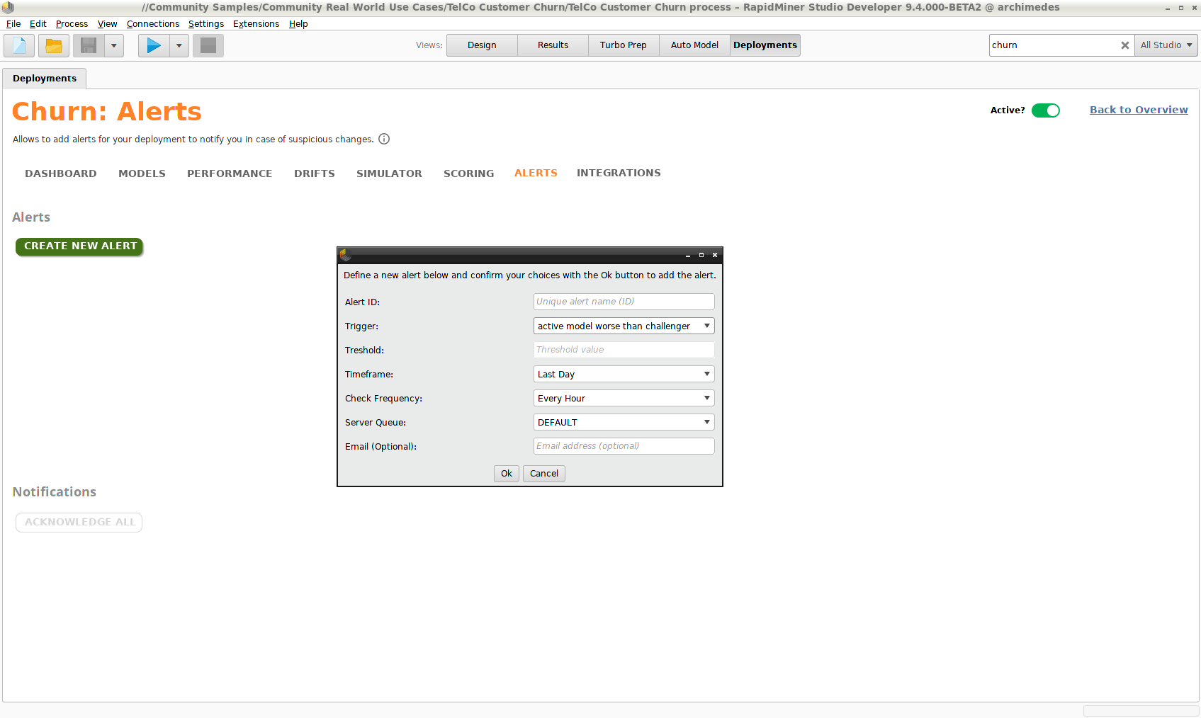
An alert warns you when there is unusual or undesired behavior in your deployment. The triggers for an alert include:
- an average error that exceeds a user-defined threshold
- average scoring times greater than a user-defined threshold
- fewer scores than expected within a given time period
- an active model that has larger errors than a challenger
- drift greater than a user-defined threshold.
To create an alert, click Create New Alert. When an alert is triggered, it will appear in the Dashboard, but you can also configure the alert to send you an email.
Integrations
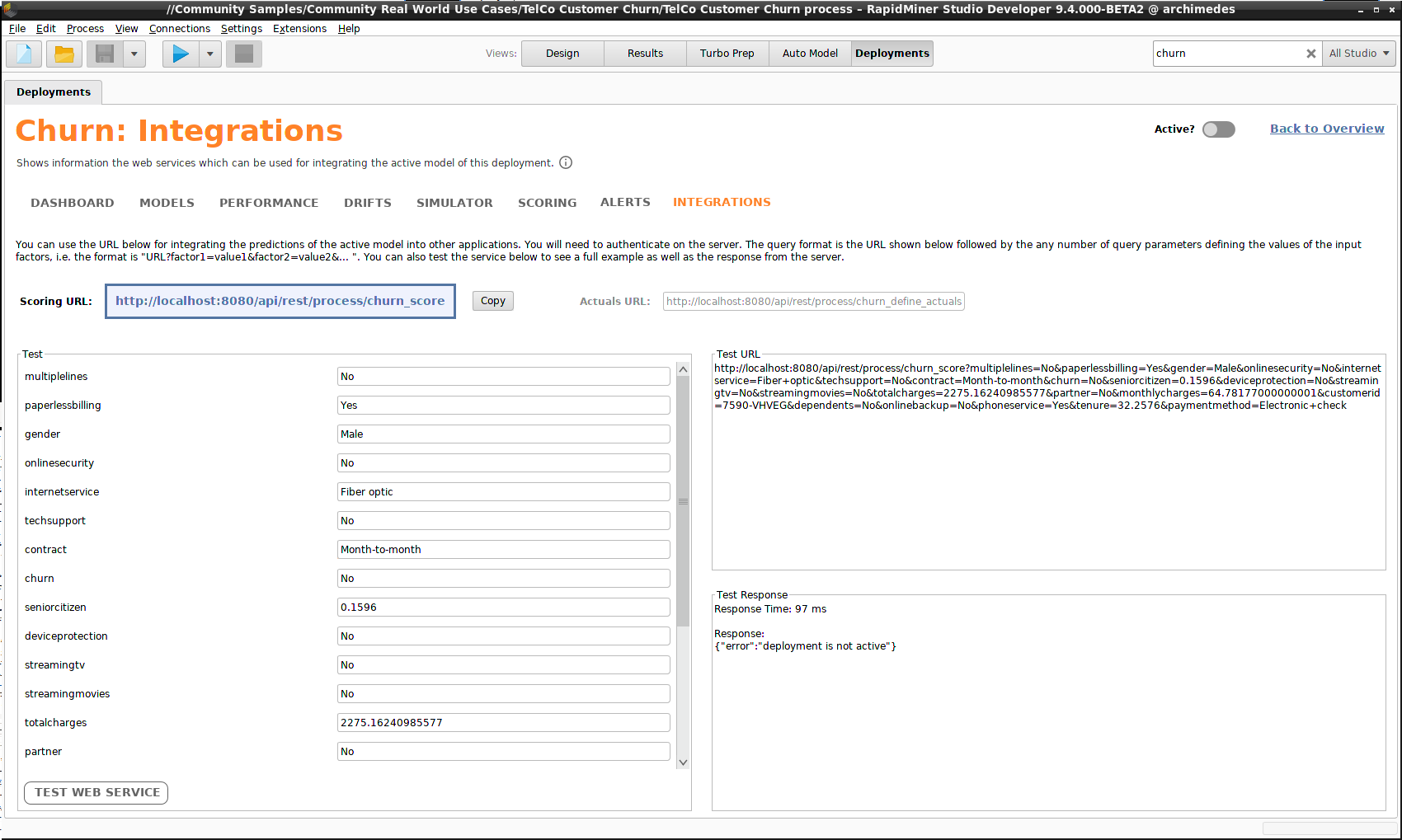
An integration is a web service that provides a Scoring URL, where you can post data for scoring. In this context, it also provides an Actuals URL, corresponding to the button Define Actuals in the scoring interface. If you're planning to automate the scoring process, a web service is precisely what you need; RapidMiner Server provides a REST API that helps you to integrate the deployment with your other software.
The Integrations component displays the Scoring URL and allows you to test it with arbitrary values of the scoring data. On the right side of the screenshot below, you can see the Test URL and the Test Response. In this example, the response from the server is "deployment is not active", because we have forgotten to flip the Active? switch on the top right of the screen, but normally the response would include a prediction with confidence values, in JSON format.
