You are viewing the RapidMiner Studio documentation for version 9.5 - Check here for latest version
Turbo Prep
Data preparation is time-consuming. You've collected data from multiple sources, in multiple formats, and now you're wondering: how do I put all the pieces together? How do I decide what's important? And how do I present my results in a way that other people can understand?
Turbo Prep is designed to make data preparation easier. It provides a user interface where your data is always visible front and center, where you can make changes step-by-step and instantly see the results, with a wide range of supporting functions to prepare your data for for model-building or presentation.
In the background, while you prepare your data, Turbo Prep builds a RapidMiner process. You can save that process and apply it later to similar data sets, so you don't have to do the same job twice.
Turbo Prep won't solve all your problems. If you want to use your data to make predictions and understand the results, see Auto Model. But you can't make predictions with worthless or inconsistent data. Turbo Prep will help you to put all the pieces together, to eliminate worthless data, to transform the remaining data into a consistent and useful format, and to present the results, once you have achieved a better understanding of your data.
Turbo Prep's supporting functions are divided into five broad categories:
- Transform - these functions help you to create useful subsets of your data (
Filter,Range,Sample,Remove) or to modify the data in individual columns (Replace). - Cleanse - these functions help you with missing values, duplicates, normalization and binning. Low quality data, of the kind discussed in Auto Model, can be removed automatically via
Auto Cleansing. - Generate - these functions help you generate new data columns from existing data columns. The large variety of logical and mathematical operators is especially useful for feature engineering and for more complex data transformations.
- Pivot - these functions simplify the task of creating summary tables (pivot tables) from your data.
- Merge - these functions help you to combine two or more data sets (
Join).
Within Turbo Prep, click on the 🛈 symbol to learn more about any of these categories.
Once you're done preparing the data, you can take additional actions, including:
- Model - Pass your data to Auto Model to help you build a model!
- Charts - Display your data using a a variety of charts.
- Process - Save your data preparation steps as a RapidMiner process, for later reuse.
- History - Examine the history of your data preparation, roll back to an earlier step, and make changes.
- Export - Save your data to a file, or save it in a RapidMiner repository.
Within RapidMiner Studio, Turbo Prep appears as a view, next to the Design view, the Results view, and Auto Model.
Example: Presenting results in a summary table
In what follows, we'll apply Turbo Prep to the Titanic data set.
Note that it is not our intention to prepare the data for model-building.
The issues with cleaning the Titanic data set are discussed in Auto Model;
Turbo Prep can clean the data in the same way via Cleansing > Auto Cleansing.
See also the video introduction to data cleansing with Turbo Prep.
Our purpose is to create a single data table that captures the essential factors relevant to survival. We assume that the results from the Auto Model documentation are known. In particular, we know that survival on the Titanic depends on the following factors:
- Sex
- Passenger Class
- Age
Auto Model makes it possible to study these factors in the context of an interactive model. Now we want to use Turbo Prep to present our results in a summary table.
Because Sex dominates the other factors in determining survival on the Titanic, and because we want to understand the role of less important factors such as Passenger Class and Age, we will split the data into two parts, male and female, and study each of the parts separately, before recombining the data at the end.
The goal is to create a table of the following form, including both male and female passengers.
Survival rate of female passengers on the Titanic
| Age | 1st class | 2nd class | 3rd class |
|---|---|---|---|
| 0-9 | 0.0 | 1.0 | 0.51 |
| 10-19 | 1.0 | 0.92 | 0.55 |
| 20-29 | 0.96 | 0.86 | 0.46 |
| 30-39 | 0.97 | 0.90 | 0.42 |
| 40-49 | 1.0 | 0.91 | 0.25 |
| 50-59 | 0.95 | 0.83 | |
| 60-69 | 0.87 | 0.0 | 1.0 |
| 70-79 | 1.0 |
To get started, choose the Turbo Prep view by pressing the button at the top of RapidMiner Studio.

Load Data
After starting Turbo Prep, the first step is to select a data set from one of your repositories.
Click
Load Data.Select the Titanic data set from the repository, under
Samples>data. (If your data isn't in a repository, selectImport Dataat the top of the screen.)Click
Load Dataonce again. Your data set now appears on the left side of the screen.
Notice that Titanic data set, once loaded, has a context (right-click) menu, with numerous options.
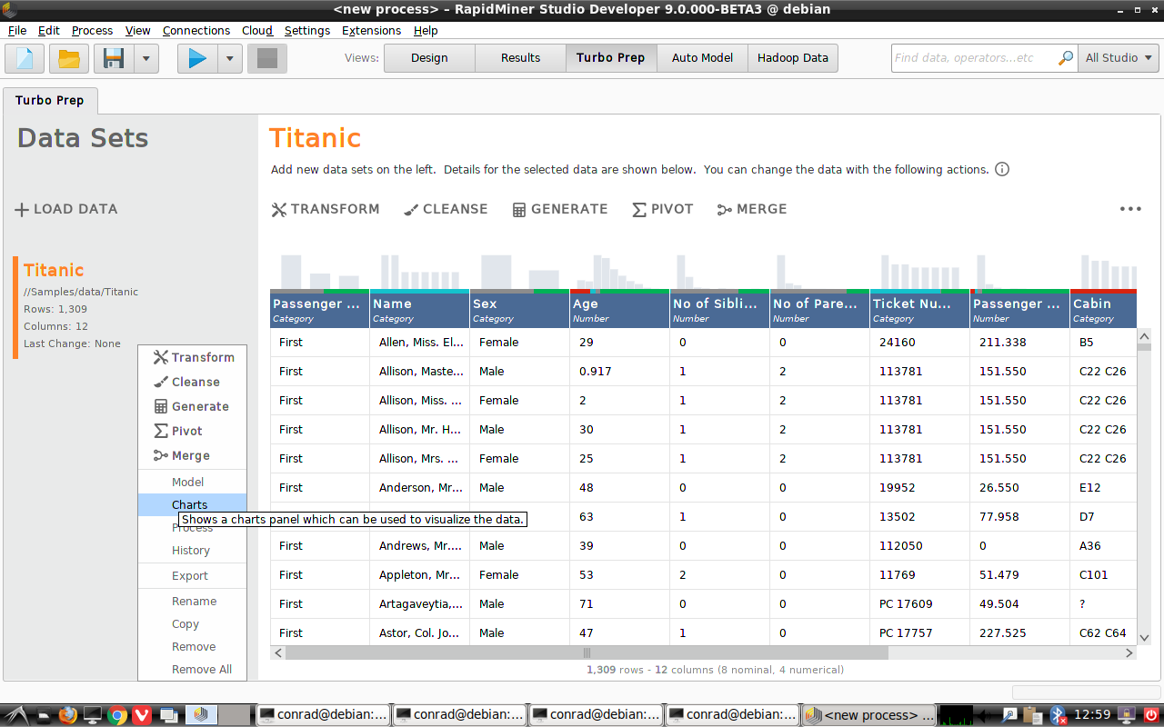
You can, for example, choose Charts with chart style Histogram Color,
and plot "Survived" as a function of "Sex" to see the difference between Male and Female survival rates:
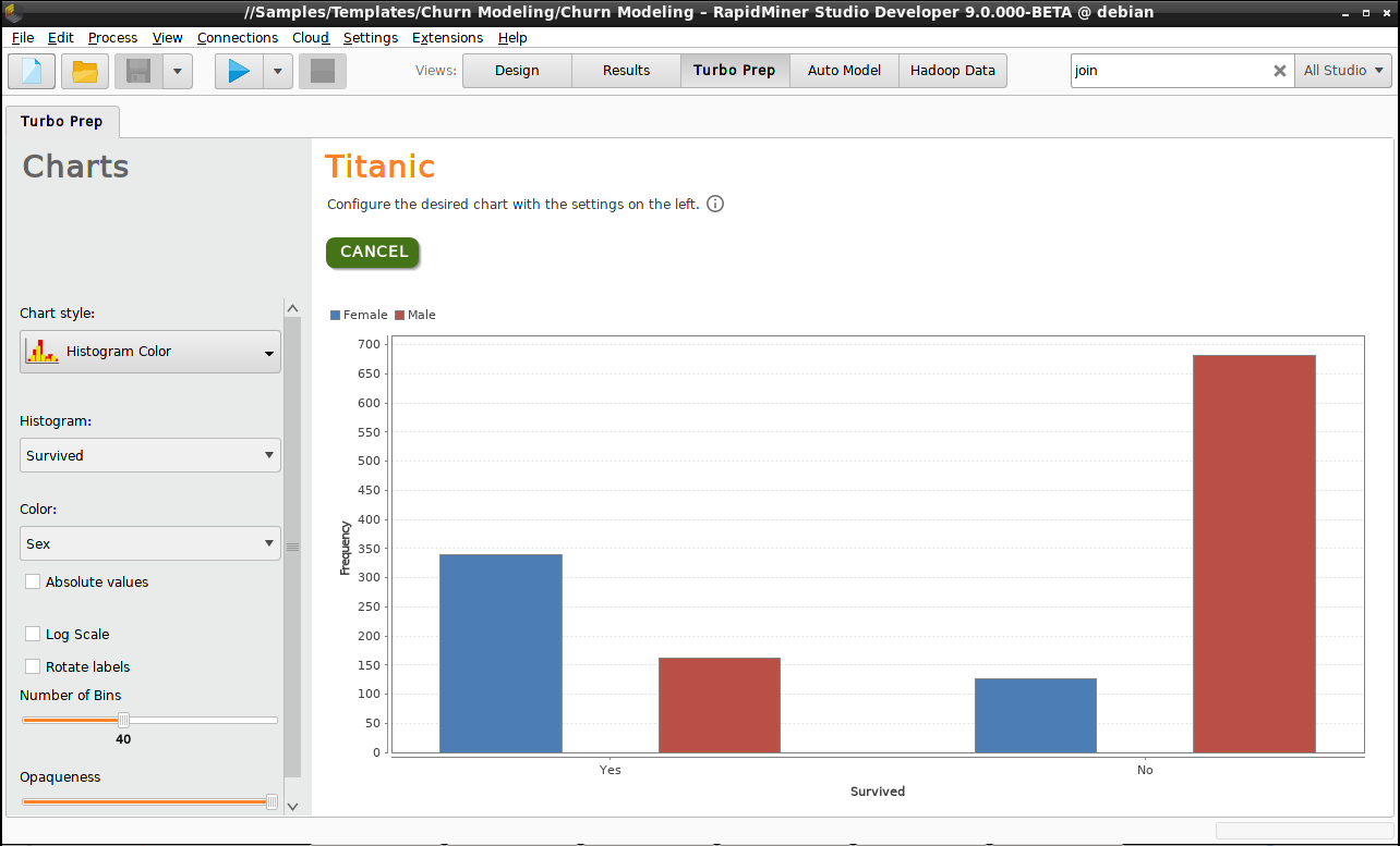
Press Cancel to leave the Chart view and return to the Data view.
Generate
At the top of the Data view, select the category called Generate.
The purpose of functions in this category is to generate new data columns based on the existing ones.
For example, the Titanic data set includes two columns called "No of Siblings or Spouses Onboard" and
"No of Parents or Children Onboard". If you were engineering new features, you might add these two columns
to generate a new column called "No of Relatives Onboard".
Generate numeric values for "Survived"
In the current analysis, we are examining survival rates, and therefore it will be useful to generate a new column based on "Survived", but with numeric values 1 and 0 instead of "Yes" and "No", so that we can more easily calculate averages and other statistics. We give the new column a name ("survived_value") and build a function in the formula editor to convert "Yes" to 1 and "No" to 0. Notice that column names from the list on the left can be dragged into the formula editor, and that function documentation is available on the right.
if([Survived]=="Yes",1,0)
Click on Update Preview to see the resulting column, and Commit Generate to save the result.
The "Survived" column is now redundant, and could be deleted (Transform > Remove), but it's not necessary.

Note: A similar result can be achieved via the function Transform > Replace
(with "Yes" replaced by 1 and "No" replaced by 0), in combination with the function
Transform > Change Type ("Change to number").
In this case, no new data column is created, and the original data column "Survived" is
converted from categorical to numerical.
Generate bins for the "Age" data
We said before that we want to understand the impact of "Passenger Class" and "Age" on survival.
To make the data more suitable for a summary table, we will put the passengers into age groups -- ages 0-9, 10-19, 20-29, etc.
To do so, we again click on Generate, give a column name ("age_category"), and build a function in the formula editor.
Notice that floor is a rounding function, so any number in the range 20-29 is rounded down to 20.
10 * floor([Age] / 10)
Click on Update Preview to see the resulting column, and Commit Generate to save the result.
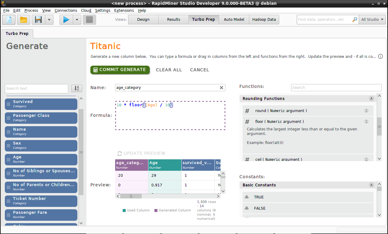
Note: A similar result can be achieved via the function Cleansing > Discretization,
by creating 8 equal-width bins for the data in the "Age" column, since the range spans 0-80 years.
In this case, no new data column is created, and the original data column "Age" is
converted from numerical to categorical, with values {range1, range2,... range8}.
Copy data
We want to make two copies of the Titanic data set and call them "Titanic_male" and "Titanic_female".
From the Data view, right-click on the Titanic data set, and choose
Copyfrom the menu.Right-click the copy, and choose
Renamefrom the menu. Call the copy "Titanic_female".Repeat steps (1) and (2) to create "Titanic_male"
Three identical data sets are now displayed in the Data view. To create male and female data sets, we need to transform the data.
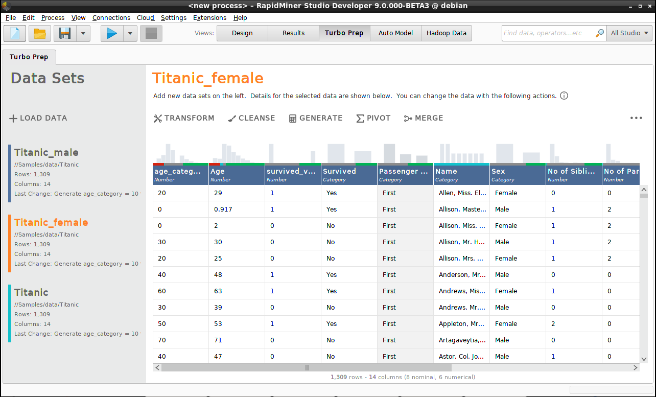
Transform
At the top of the Data view, select the category called Transform.
For the data set called "Titanic_female", our purpose is to keep all
the data related to female passengers, discarding all the data related
to male passengers.
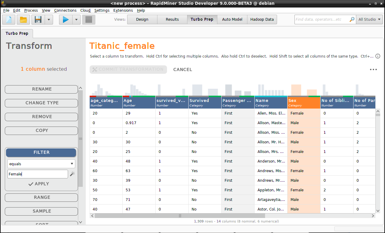
Click on the data column named "Sex".
Select
Filterfrom the list of functions on the left. Choose "equals" for the relationship, and "Female" for the value. ClickApply.Click
Commit Transformation.
Once the transformation of "Titanic_female" is complete, repeat the operation for "Titanic_male", using the value "Male" in the Filter function.
Pivot
See also the video introduction to data pivoting with Turbo Prep.
At the top of the Data view, select the category called Pivot. A pivot table is a summary data table.
Usually the rows and columns are composed of categories from your original data set,
while the individual cells contain numeric data, typically in the form of a sum (e.g., "Total Sales")
or an average (e.g., "Survival Rate") for all the data points belonging to those categories.
With Turbo Prep, creating a pivot table is easy: drag a column name from the left, and drop it onto one of the three boxes:
Group-By- The data categories you choose here will become rows in your pivot table.Column Grouping- The data categories you choose here will become columns in your pivot table.Aggregates- The numeric data you choose here will typically be summed or averaged.
Take the following steps for each of the data sets "Titanic_female" and "Titanic_male":
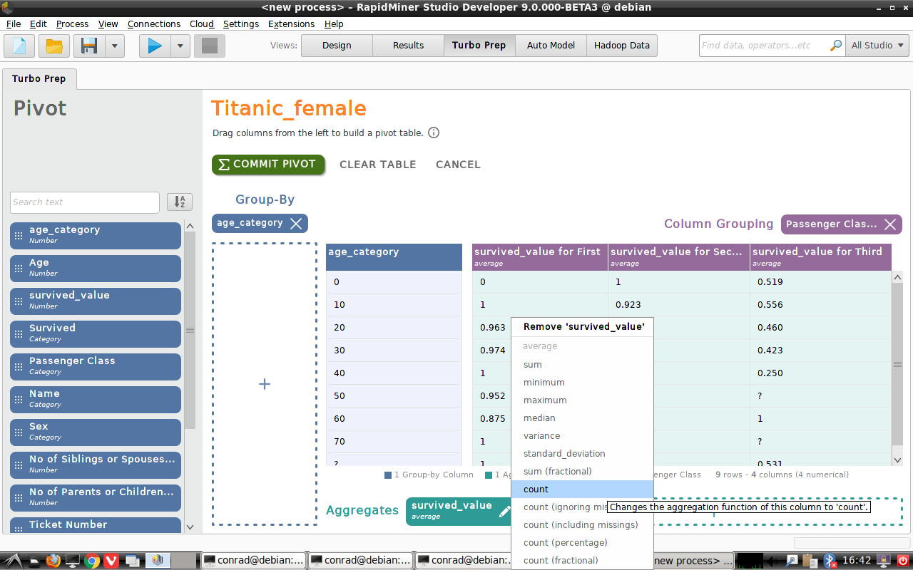
Drag "survived_value" into
Aggregates. This first version of the pivot table is composed of a single value, the survival rate for all females (males).Drag "Passenger Class" into
Column Grouping. The pivot table now has 3 cells, with a survival rate for each passenger class.Drag "age_category" into
Group-By. The pivot table now includes the survival rate for females (males) in each of several categories, sorted according to age (rows) and class (columns).
In our example, the the survival rate is calculated by taking the average of "survived_value" for each cell in the pivot table, but notice that you can right-click on "survived_value" and choose a different statistic, such as "sum" (to get the number of passengers that survived) or "count" (to get the total number of passengers).
When you're done creating the pivot table, click Commit Pivot.
Results
Examining the two pivot tables for "Titanic_female" and "Titanic_male", we can draw some conclusions:
Among female passengers, those in first and second class had a significantly better chance of survival than those in third class (90% vs 50%).
Among male passengers, those in first class had a significantly better chance of survival than those in second or third class (35% vs 15%).
Male passengers in third class were actually more likely to survive than those in second class, unless they were small children.
Passengers above the age of 40 were less likely to survive than younger passengers, with the exception of females in first and second class.
The survival rate for female passengers was given in the table above.
Survival rate of male passengers on the Titanic
| Age | 1st class | 2nd class | 3rd class |
|---|---|---|---|
| 0-9 | 1.0 | 1.0 | 0.37 |
| 10-19 | 0.42 | 0.06 | 0.08 |
| 20-29 | 0.44 | 0.09 | 0.19 |
| 30-39 | 0.41 | 0.09 | 0.17 |
| 40-49 | 0.32 | 0.05 | 0.06 |
| 50-59 | 0.28 | 0.0 | 0.0 |
| 60-69 | 0.07 | 0.16 | 0.0 |
| 70-79 | 0.0 | 0.0 | 0.0 |
| 80-89 | 1.0 |
Merge
See also the video introduction to merging data with Turbo Prep.
We now want to merge the two pivot tables, "Titanic_female" and "Titanic_male".
Unfortunately, the two pivot tables have a nearly identical structure, and only
the name of the data set makes it clear which data is male and which is female.
To avoid losing important information, we rename (Transform > Rename)
the 3 passenger classes to {female1, female2, female3} in "Titanic_female" and
to {male1, male2, male3} in "Titanic_male".
Then we create a new pivot table called "Titanic_merged".
Right-click "Titanic_female" and choose
Copy.Right-click the copy and choose
Rename. Call the new data set "Titanic_merged".
At the top of the Data view, select the category called Merge.
The idea of a "join" is that each row of data can be identified by a unique "key";
when two rows in the two data sets have the same key, their data is combined.
A complication occurs when a key occurs in one data set, but not the other.
Then you have to decide whether that data should be included in the combined table -- or not.
| Method | Include the data in the combined table... |
|---|---|
| Inner Join | ...only if the key appears in both data sets |
| Left Join | ...only if the key appears in the first data set |
| Right Join | ...only if the key appears in the second data set |
| Outer Join | ...if the key appears in either data set (all data) |
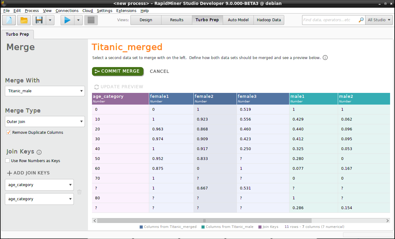
In our example, the "join keys" are the values of "age_category", but "Titanic_male" includes a passenger who is 80+ years of age, while there is no such passenger in "Titanic_female". With an inner join or a left join, we will lose this data; to include it, we must choose a right join or an outer join. The surest way to include all data is to use an outer join.
- Merge With - "Titanic_male", since our starting point was "Titanic_female"
- Merge Type - "Outer join", so no data is lost
- Join Keys - "age_category"
Click on Commit Merge.
Notice that "Titanic_merged" includes rows where the "age_category" is missing.
You can delete them by clicking on "age_category", followed by
Transform > Filter > "is not missing".
Additional actions (⋯)
What's left to do? We've succeeded in generating a pivot table for survival rate on the Titanic, measuring the impact of "Sex", "Passenger Class", and "Age", with the results now contained in a single table.
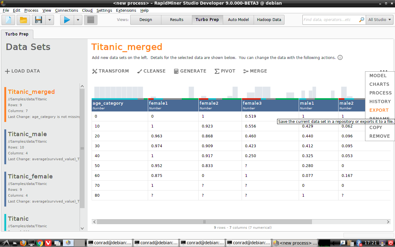
The additional actions menu (⋯) on the top right of the Data view gives some hints.
Export
You can save the final pivot table to a file or to a RapidMiner repository. The available file formats include Excel (.xlsx), CSV (.csv), and Qlik (.qvx).
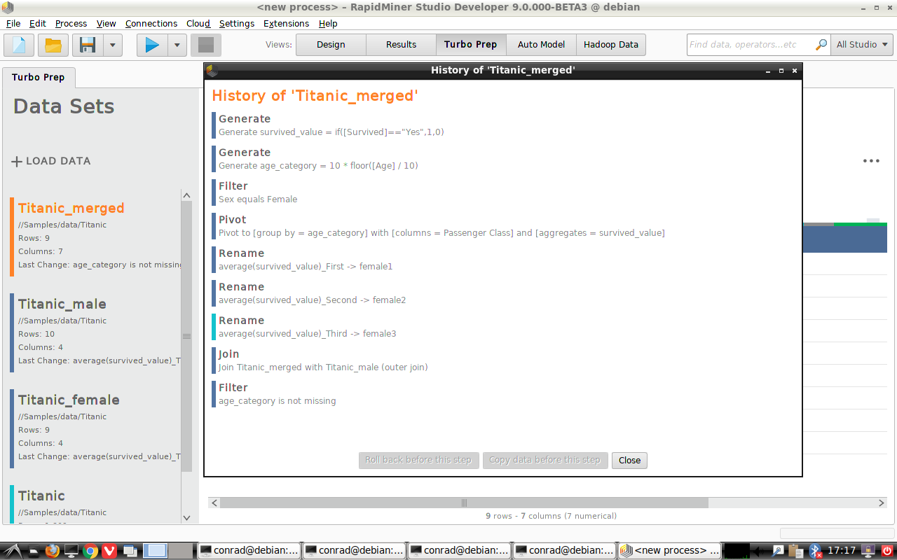
History
You can examine the history of your data preparation, roll back to an earlier step, and make changes.
Model
It's not relevant in our current example, but if we had been preparing our data for model-building, the next step might have been to pass it to Auto Model.
Process
It's not relevant in our current example, but if a new version of the data set were generated once weekly, we could generate a weekly summary table by saving our work as a RapidMiner process, then feeding the new data sets to that process.
Charts
You can display your data using a a variety of charts.