You are viewing the RapidMiner Studio documentation for version 9.9 - Check here for latest version
Install the Deep Learning extension
Disclaimer: This documentation is about setting up and using the RapidMiner Deep Learning extension. These paragraphs will not explain the concept of Deep Learning.
Table of contents
Do I need a GPU?
It's impossible to discuss the topic of Deep Learning without first pointing out that -- at least for large data sets -- you're probably better off if you have access to one or more CUDA-capable GPUs, either:
- on your computer,
- on RapidMiner AI Hub, or
- in the cloud.
But if your data set is smaller, or you simply want to become familiar with the Deep Learning extension, you don't need a GPU. All you need to do is to install, within RapidMiner Studio, the following two extensions from the RapidMiner marketplace:
plus (optionally) any additional extensions that may be relevant to your application, for example:
Install the same extensions on RapidMiner AI Hub, if you plan to run your processes there.
If you're not going to use a GPU -- at least not yet -- you are now ready to go! No additional software is needed. Make sure to check out the in-product help texts for the Deep Learning operators and look at the sample processes provided in the repository under Samples/Deep Learning. You can skip ahead to the Introduction.
ND4J Back End
If you want to go beyond the minimal (default) setup described above, to achieve better performance, you will need to install additional software. Note that the ND4J Back End extension provides and configures the computational back end for training and scoring neural networks. Currently three back ends can be selected:
CPU-OpenBLAS (default): The default back end uses the CPU of the machine where the processes are executed; the OpenBLAS library is used for calculations. You do not need to install additional software. Choose this option for initial network setup and testing on smaller data sets in RapidMiner Studio.
CPU-MKL: This option uses Intel's MKL library to speed up calculations on the CPU; it is recommended if an Intel MKL-supported CPU is available, but no GPU. You need to install the Intel Math Kernel Library.
GPU-CUDA: This option provides accelerated calculations on one available GPU. After checking that your GPU is compatible, you need to install NVIDIA's CUDA version 10.1. If the GPU also supports the GPU acceleration library cuDNN (version 7.6), we recommend that you install it for enhanced performance.
For both the CPU-MKL and the GPU-CUDA back end, make sure that the libraries you installed
are available on the classpath, e.g. by adding them to the LD_LIBRARY_PATH environment variable.
Read more: Settings
CUDA and cuDNN
If you plan to use the GPU together with RapidMiner Studio, you need to install NVIDIA's CUDA version 10.1 and cuDNN version 7.6.
For users of RapidMiner AI Hub, we provide an alternate path, via Docker images specially configured for Deep Learning. On these GPU-capable Docker images, CUDA and cuDNN are pre-installed and pre-configured.
Introduction to the Deep Learning extension
The RapidMiner Deep Learning extension enables creation and usage of sequential neural networks, but not (yet) non-sequential neural networks. Networks can be created inside the nested Deep Learning or Deep Learning (on Tensor) operators, by appending layer operators one after another. The layer operators are all named Add <LayerType> Operator, where <LayerType> is the type of layer, e.g.:
- fully-connected
- CNN
- LSTM
In contrast to other RapidMiner operators, it is not possible to obtain the intermediate output of a layer operator by setting a break point. These layer operators are just used for configuring the network architecture and hence provide only the architecture configured up to that point on their output port.
It is not necessary to add layers for dimensionality handling and rarely necessary to define the input shape of the data manually, since this is done automatically in the background, so no flattening layers are needed.
General parameters like the number of epochs or early-stopping mechanisms to train are set as parameters of said nested Deep Learning operators, while the individual layer settings like the number of neurons or activation function to use are set for each layer with the respective Add <LayerType> Layer operator. There is one exception: bias and weight initialization. Choosing the method for initializing bias and weight values layers can be done either centralized from the Deep Learning operator to set it for all layers alike, or individually by choosing the overwrite networks weight/bias initialization parameter for a given layer operator.
Layer weights and biases as well as the logged scores from provided training and potentially test data can be obtained through the output ports of the Deep Learning operator. In addition, you can monitor the scores live via the logs of RapidMiner Studio or RapidMiner AI Hub, or via a provided web interface.
The Deep Learning extension allows for different computational back-ends to work in different CPU and GPU environments. These back-ends are made available through the dependent back-end extension called ND4J Back End. This extension also allows setting of certain memory handling parameters. While network creation and usage utilizing the CPU works on Windows, macOS and most Linux distributions alike, for GPU calculations only Windows and Linux are supported for NVIDIA GPUs working with CUDA 10.1.
As the name of the back-end extension already hints, both the Deep Learning and the back-end extension are based on the DeepLearning4J project suite. DeepLearning4J (DL4J) is an open-source project providing libraries for numerical computations incl. computational back-end handling as well as deep learning functionality and more. The currently used DL4J library version is always stated in the release notes.
Settings
Here we discuss the settings for the Deep Learning / ND4J Back End extensions in RapidMiner Studio.
See also: Settings for Deep Learning / ND4J Back End on RapidMiner AI Hub
Computational back ends
As discussed above, the Deep Learning extension needs the ND4J Back End extension to function, since it provides and configures the computational back ends to be used for training and scoring neural networks.
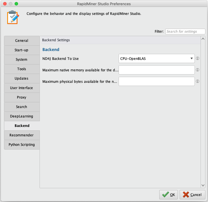
In RapidMiner Studio, open the Preferences dialog under Settings > Preferences, select Backend, and set the ND4J Backend To Use from the following values:
- CPU-OpenBLAS (default)
- CPU-MKL
- GPU-CUDA
Memory limits
Because the calculations needed for training and scoring are performed outside the Java Virtual Machine (JVM), it is recommended to limit the memory that is used.
In RapidMiner Studio, open the Preferences dialog under Settings > Preferences, select Backend, and set the Maximum native memory available for the deep learning backend:
Training UI Port
You can monitor currently running training processes via a web browser, if you configure a port for a training UI. Information displayed includes the epochs and their respective scores calculated on the training data and the test data, in case the latter was also provided, as well as metadata about the layer architecture.
In RapidMiner Studio, open the Preferences dialog under Settings > Preferences, select DeepLearning, and set the DeepLearning Training UI Port:
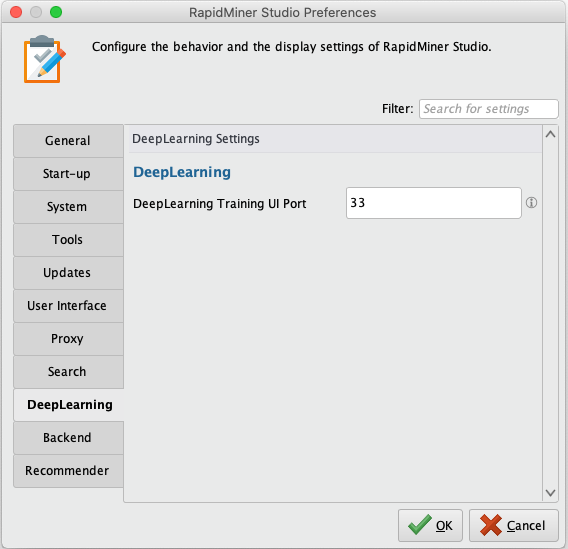
To access the training UI, open a browser and enter localhost as the URL
(or your computer's IP address), followed by a colon, followed by the
configured port number (e.g., localhost:33).
Data handling - tensors and dimensionality
Neural networks can be applied not only on two dimensional tabular data like a RapidMiner ExampleSet, but also on images, text, three dimensional data like multivariate time-series and more. Depending on the type of data, different preparation steps are necessary, since neural networks require numerical data in tensor form and often benefit from normalization.
RapidMiner offers plenty of options to preprocess data sets. This section will give some hints regarding helpful mechanisms to be used for certain data types and explain how the Deep Learning operators handle dimensionality and how data stored in the cloud can be leveraged.
Note that there are two Deep Learning operators: one for tabular data (ExampleSets) and one for tensor data (here mostly: Images, Text and Time-Series). Note we're using the term "tensor data" as a synonym for three-dimensional arrays, in contrast to the regular ExampleSets found in RapidMiner that are two-dimensional arrays.
- Deep Learning operator - accepts only ExampleSets as input
- Deep Learning (Tensor) operator - accepts all other types of data
Note also that there are two different versions of the Apply Model operator:
- Apply Model - use together with models created by Deep Learning
- Apply Model (Generic) - use together with models created by Deep Learning (Tensor) or Deep Learning.
Input shape / up-scaling / down-scaling
Both Deep Learning operators try to infer the input shape of the data by default. This works in many cases. If the desired input shape is not recognized, disable the advanced parameter infer input shape, select a network type you are setting up and fill in the new parameters allowing you to enter values for given dimensions.
Inside the network the up- and down-scaling of dimensions between certain layers is done automatically.
Extra layers for up-sampling to create Decoders or the like are not yet available.
ExampleSets
ExampleSets are two-dimensional arrays, where just rows and columns are available. The Deep Learning operator handles it natively. It is possible to provide nominal labels as dummy encoding is performed automatically. Make sure to convert all other columns into a meaningful numerical representation to ensure that neural networks can be trained and applied. E.g. use the Nominal to numerical, Parse Numbers or other operators to convert all non-special attributes to numerical ones.
Sequential Data (e.g. Time-Series)
Sequential data has the distinct difference in comparison to non-sequential data, that the actual ordering of entries is of importance. Hence providing an ordered ExampleSet is necessary. It is possible to provide series-like data in two forms.
Option 1
The ExampleSet to Tensor operator accepts one long ExampleSet with two columns as input, where one column is used to assign a batch ID that assigns each Example to a given sequence, while the second ID identifies the ordering in the given sequence. This option is recommended, for example when reading time-series data from a database.
Example: Having a time-series with 5 measurements of 10 tensors, where each measurement contains 20 time-steps would result in an ExampleSet with 100 examples (rows) and 12 attributes (columns). Two attributes would be said ID attributes, while the remaining 10 represent sensor readings. The batch ID would contain entries from 1 to 5, whereas each entry would occur 20 times. Whilte the sequence ID could be counting from 1 to 20, 5 times. It is also possible to have varying sequence length between batches, so different number of entries per batch. The masking of the data needed for the neural network is performed automatically.
Option 2
The TimeSeries to Tensor operator accepts a collection of ExampleSets as input, where each Example in a given ExampleSet represents a part of the sequence e.g. a time-step or a token of text, while each ExampleSet represents one whole series. For this option no creation of an ID column is needed. The series ID is taken from the ordering of each given ExampleSet. It is also possible to have ExampleSets of varying length representing a varying number of sequence entries. The masking of the data needed for the neural network is performed automatically.
Currently network training for many-to-one and many-to-many scenarious are
supported. Both mentioned operators infer the sequence type from the label
being constant or not. This option can be overwritten.
many-to-one is used e.g. for classification scenarious, where one value
should be predicted for a sequence of entries, while many-to-many can be
used, when multiple predictions should be made, given a sequence input.
Text
See the extensions Text Processing and Word2Vec
Neural networks require numerical data for their internal calculations. Hence text first has to be converted into a numerical representation. Converting text to a numerical representation is often done using word embeddings like Word2Vec, GloVe or others. These embeddings are pretrained representations, that are trained on text corpora to provide a numerical vector per word it was trained on. To convert text using these embeddings, first the text needs to be tokenized (e.g. using operators from the Text Processing extension). Afterwards the "Text to Embedding ID" operator can be used to convert each token into the ID it has in the dictionary of a chosen embedding. This ID is later converted into a numerical vector inside the neural network. Thus adding an embedding layer as the first layer to the network is necessary. After scoring a data set, these IDs can be converted back to their respective token.
Word embeddings can be downloaded from various sources, or created on own corpora e.g. using the Word2Vec extension. In most cases it is recommended to use existing embeddings.
Images
See the extension Image Handling
Images can be read and pre-processed using the Image Handling extension. This extension provides operators to read in a list of image paths from a directory using the folder names as labels. These paths are later used to access the images and perform pre-processing steps on them, just before they are needed for training.
The Pre-Process Images operator has a tensor output port that can be fed into the Deep Learning (Tensor) operator to obtain numerical representations of provided images, that can be used by the network.
Make sure to use the Group Model (Generic) operator to combine the pre-processing model from the Pre-Process Images operator with a trained Deep Learning model to obtain one single model, that can be applied on unseen images.
Cloud Data
Accessing a large number of images is often done from cloud storage locations like Amazon S3 or Azure Data Lake. Use the Read Amazon S3 and Read Microsoft Data Lake Storage operators from RapidMiner Studio to access the images and write them to a persistent volume connected to the docker image used for the GPU-enabled Job Agent. Afterwards, use the Read image meta-data operator to read those images from the persistent volume, saving time and bandwith when iterating over various parameters to fine tune the network.
Model Import (Keras)
The Deep Learning extension allows you to import models created with Keras (both the original multi back-end Keras and Tensorflow Keras). Currently the import is limited to sequential models though.
In order to use Keras models inside RapidMiner, export them via Keras' save_model
function to an hd5 file that contains both the architecture and the weights.
Afterwards, this model file can be read using the Read Keras Model operator.
This operator converts the model into a native DL4J model, that can be applied inside
RapidMiner using the Apply Model operator without having to have Python installed.
If a classification task was performed, it is possible to define nominal values for used numerical representations of the class values through the operators parameters.
Workflow for training in the cloud
- Typically for Deep Learning, model training on a GPU is desired. You can deploy RapidMiner's Deep Learning template on a cloud service provider of your choice.
- Create your first network as a process in RapidMiner Studio and test it locally.
Prepare the process for training on a GPU:
- Set up cloud data access, as discussed above.
- Make sure to persist results by using a store or write operator of your choice.
- Increase batch sizes to take advantage of the memory available from a GPU.
- Make sure to set early stopping mechanisms to stop training as soon as your requirements are met.
- Move the training process to your RapidMiner AI Hub instance and execute it on a GPU-enabled Job Agent.
- Optional: Monitor the training scores live via a training UI port.