You are viewing the RapidMiner Go documentation for version 9.5 - Check here for latest version
Inspect models
RapidMiner Go is being discontinued. For an alternative, please contact sales about our new AutoAI cloud solution.
Results
In the first 4 steps of RapidMiner Go, you may have clicked your way through. Now you need to slow down and assert your expertise. At first sight, the results may seem overwhelming, so don't lose sight of the purpose:
to help you identify the most useful models (see Performance metrics and Model comparison)
to help you better understand your models and data (see Weights and Model Simulator)
to make predictions, after you have completed steps (1) and (2)
If you're looking for a user-friendly starting point, have a look at the Model Simulator.
While it may be tempting to treat your model as a black box, plug in new data, and make a prediction, the output of a black-box prediction can be misleading -- see the summary of the Churn example.
Table of contents
Performance metrics
To say whether a model is good or bad, and in particular whether it is better or worse than some other model, we need to have some basis of comparison. By assigning a numeric measure of success to the model, a so-called performance metric, you can compare it with other models and get some idea of its relative success.
The complication is that many different performance metrics exist, and none of them is absolute as a standard of success; each has strengths and weaknesses, depending on the problem you're trying to solve. You will have to choose the best performance metric for your problem, and with the help of this performance metric, you can choose the best model.
To calculate the performance metrics, we start by building a model based on a random sample of 80% of your data (the training set). Once it is built, we apply the model to the remaining 20% of your data (called the test set) and compare the predictions with the known values. Ideally there should be no difference, but in practice there usually is, because the predictions are rarely 100% correct.
Recall from 2. Choose column that the type of problem you're solving depends on the values in the target column. Are they categorical or numerical? Depending on what you're trying to predict, there are different performance metrics. For a more detailed discussion, including examples, see the links below:
- 5A. Binary classification (categorical data, two possible values)
- 5B. Multiclass classification (categorical data, three or more possible values)
- 5C. Regression (numerical data)
Model comparison
Once you have chosen a performance metric, you can use the model comparison to help you find the best model, according to that metric.
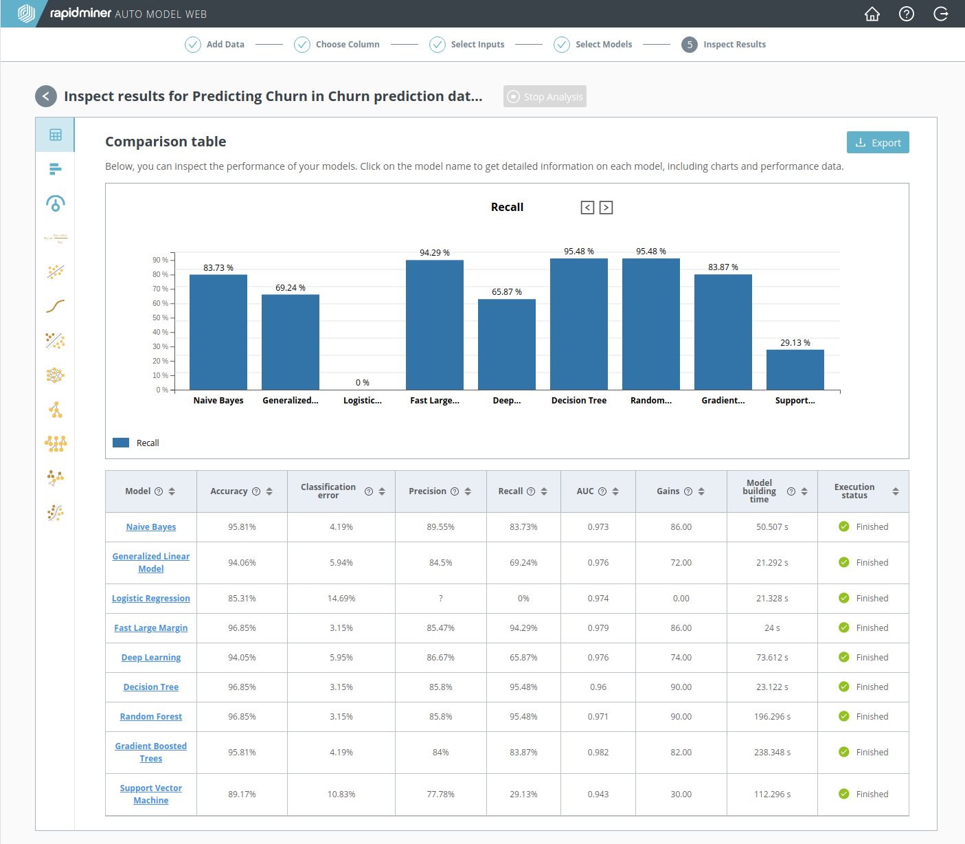
The model comparison displays the performance of each model:
- as a bar chart, for any particular performance metric, comparing the models head-to-head
- as a table, with models as rows and performance metrics as columns
Click on a performance metric to display the bar chart for that metric. Click on a model to learn more about the details of that model. As discussed in 5A. Binary classification, Recall is the most useful metric for the Churn Prediction Data, and according to that metric, the models with the best performance are Decision Tree and Random Forest.
Weights
Click on the Weights icon to learn more about your data, independent of the model. The Weights tell you which input data is mostly likely to affect the prediction. From 3. Select inputs, we knew already that "CustServ Calls" was the most important column in the Churn Prediction Data. The Weights show that "Intl Plan", "Day Mins", and "Day Charge" are the next most important columns, although their weight is much less.
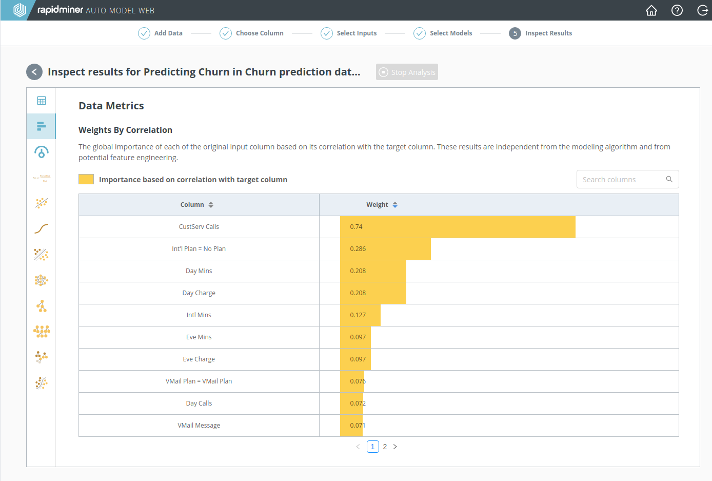
In the Model Simulator, change the values of the input data with the highest weights, and you will quickly understand the importance of that data. Input data with a lower weight is less likely to have an impact.
Model Simulator
RapidMiner Go not only helps you to get results; it also helps you to understand those results. To get a better insight, click the Model Simulator icon, and select a model. We select Decision Tree, since the Model comparison identified it as a good model, and it's relatively easy to interpret.
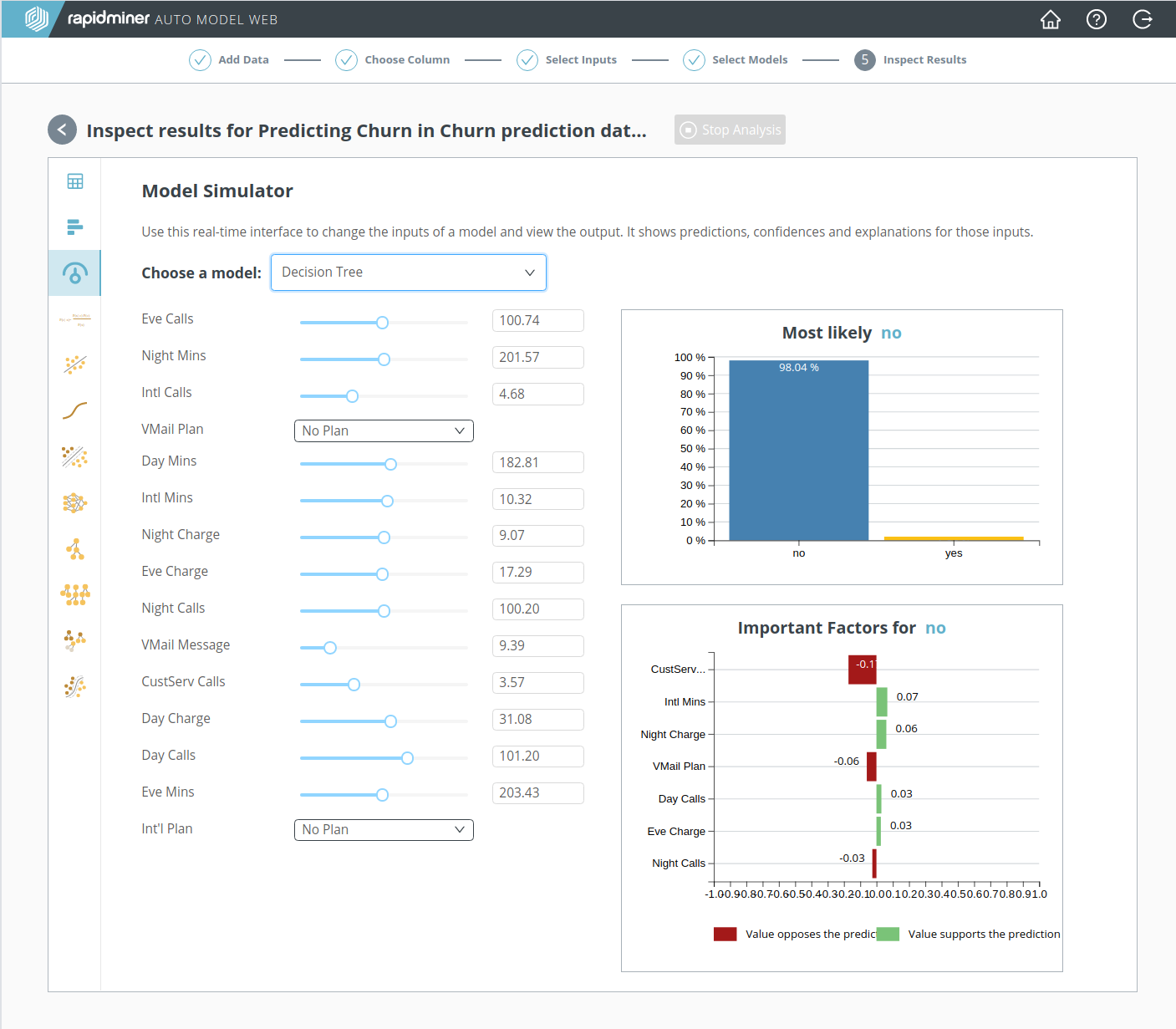
The beauty of the Model Simulator is that it is interactive, so you can change all values at will, and immediately see the impact on predictions. By manipulating all the sliders and dropdown lists, you can quickly build some intuition for the model, even hard-to-interpret models such as Deep Learning.
For its initial state, the Model Simulator chooses average data values, displayed on the left. On the right, a prediction is displayed ("no", the average customer will not churn), together with important factors. At the top of the important factors is "CustServ Calls", the data column with the highest weight, whose high correlation with the target column was identified even before we built any models, under 3. Select inputs.
By moving the slider for "CustServ Calls" back and forth from its initial value at 3.57, we can therefore expect to learn something. Notice in particular that when the value of "CustServ Calls" increases to 7.00, the prediction flips from "no" to "yes". Conclusion? Too many phone calls to customer service, and the customer will churn! None of the other sliders has the same impact.
The transition from "no" to "yes" occurs rather abruptly, when the value of "CustServ Calls" is between 6 and 7, but there is an indication of trouble even before then, described in the Important Factors. You can think of it as a protest vote. As "CustServ Calls" increases to 7.00, it opposes the "no" prediction more and more strongly, finally reaching a value of -0.87 in the Important Factors, before the prediction changes to "yes". Then the protest is over, and "CustServ Calls" agrees with the prediction.
| CustServ Calls | Prediction | Important Factor (CustServ Calls) |
|---|---|---|
| 2.00 | no (98.04%) | 0.0 |
| 3.00 | no (98.04%) | 0.0 |
| 4.00 | no (98.04%) | -0.28 |
| 5.00 | no (98.04%) | -0.55 |
| 6.00 | no (98.04%) | -0.79 |
| 6.50 | no (83.55%) | -0.86 |
| 6.90 | no (54.56%) | -0.87 |
| 7.00 | yes (59.93%) | +0.87 |
| 7.20 | yes (74.42%) | +0.86 |
| 8.00 | yes (74.42%) | +0.75 |
Continue with the Example: Churn Prediction Data
Export
RapidMiner Go is not a black box. From the details view of each individual model, you can Export a copy of the RapidMiner process that created it, and you can import that process into RapidMiner Studio for more detailed examination. There you can run the process, you can modify the process, you can make any changes you like!